
Geometric Distribution
What Is a Geometric Distribution?
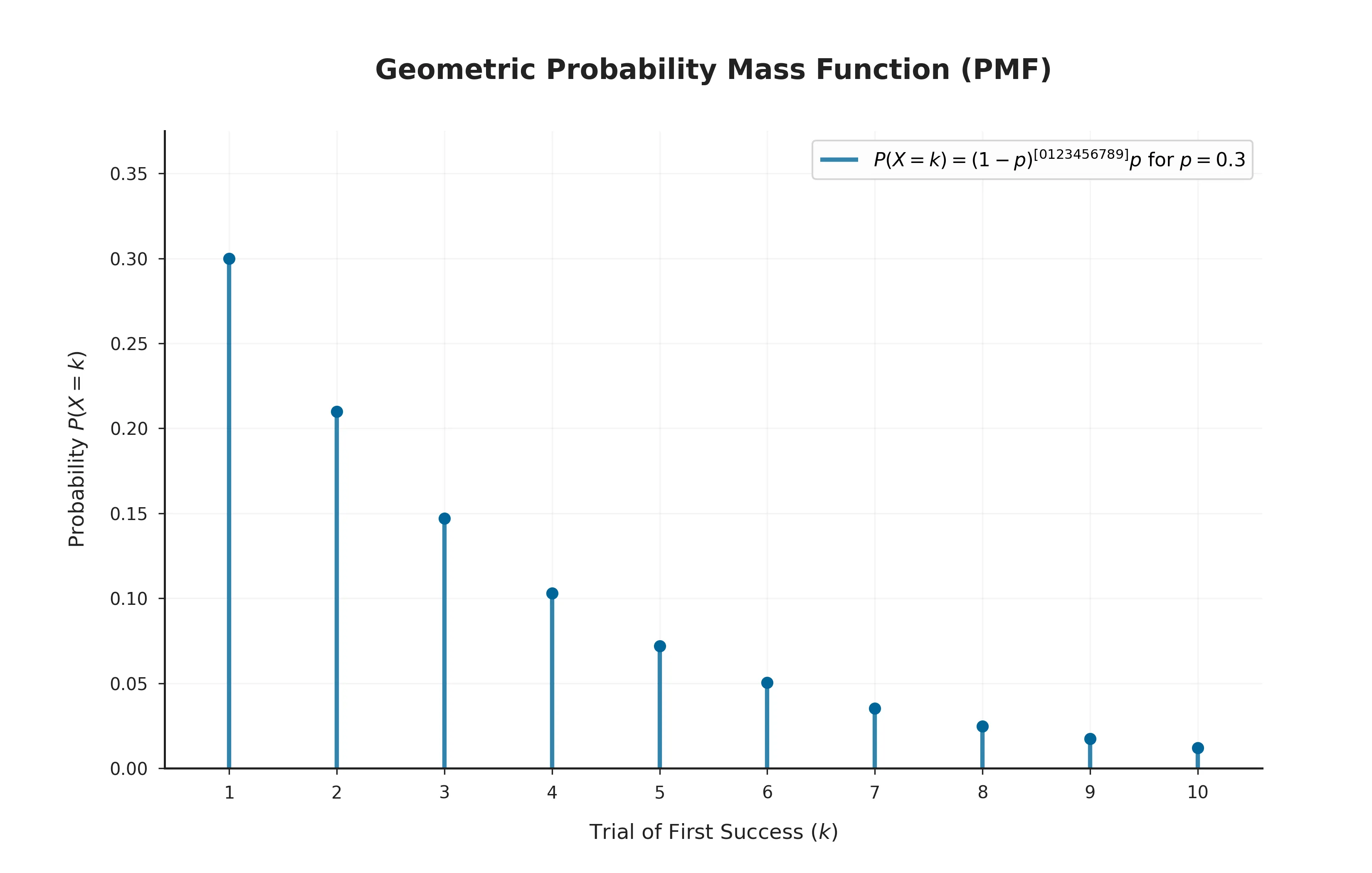
In probability theory and statistics, the geometric distribution is the discrete probability distribution of the number of independent trials needed to obtain the first success, where each trial has only two possible outcomes - success or failure - and the same success probability \( p \) on every trial. It answers a different question from the binomial distribution: instead of fixing the number of trials \( n \) in advance and counting successes, the geometric distribution fixes the target at one success and lets the number of trials itself be random. See the formula below for the precise mathematical definition.
Each individual trial that makes up a geometric experiment is itself a Bernoulli trial, and the geometric distribution describes the count of such trials repeated, one after another, until the first success interrupts the run of failures. This makes it a natural model for waiting: the number of coin flips until the first head, the number of sales calls until the first sale, the number of attempts a network makes before a packet is successfully delivered (see Where It Shows Up).
The Formula
The probability mass function (PMF) of a geometric distribution, which gives the probability that the first success occurs exactly on the \( k \)-th trial, is:
\[ P(X = k) = (1-p)^{k-1} p, \qquad k = 1, 2, 3, \ldots \]The formula has a direct interpretation: the first \( k-1 \) trials must all fail, an event with probability \( (1-p)^{k-1} \) by independence, and the \( k \)-th trial must succeed, with probability \( p \). Multiplying these two independent events together gives the probability of that exact sequence - fail, fail, …, fail, success.
A second, equally common convention defines \( Y \) as the number of failures before the first success, so that \( Y = X - 1 \) takes values \( 0, 1, 2, \ldots \) with PMF \( P(Y=k) = (1-p)^k p \). The two versions carry identical information and differ only by a shift of one; this article uses the "trials until first success" convention, \( k = 1, 2, 3, \ldots \), unless stated otherwise, but it is worth checking which convention any given textbook or software library uses before comparing formulas.
Notation & Parameters
A geometric distribution with success probability \( p \) is written compactly as:
\[ X \sim \operatorname{Geometric}(p) \]read as "\( X \) follows a geometric distribution with success probability \( p \)." A single parameter fully specifies the distribution:
- \( p \) is the success probability on each individual trial, satisfying \( 0 < p \le 1 \), and identical across every trial in the sequence.
- The support of the distribution - the set of values \( X \) can take - is the infinite set of positive integers \( \{1, 2, 3, \ldots\} \) under the "trials until first success" convention, making the geometric distribution discrete and, unlike the binomial distribution, unbounded above: in principle, the first success could take arbitrarily many trials to arrive.
- The two defining assumptions - independence across trials and an identical success probability \( p \) on every trial - mirror the i.i.d. assumptions underlying the binomial distribution. If \( p \) itself drifts from trial to trial, or trials are not independent, the resulting count is no longer exactly geometric.
Core Properties
The geometric distribution's descriptive properties - mean, variance, skewness, kurtosis - all follow from summing an infinite geometric series, the source of the distribution's name.
Mean (Expected Value)
The expected value of a geometric random variable, representing the average number of trials needed to see the first success, is:
\[ E[X] = \frac{1}{p} \]Intuitively, a rarer success (smaller \( p \)) requires waiting through more trials on average, and the relationship is inversely proportional: halving \( p \) doubles the expected number of trials needed. A fair coin (\( p=0.5 \)) takes two flips on average to see the first head; a success probability of \( p=0.1 \) requires ten trials on average.
Variance
The variance of a geometric random variable is:
\[ \operatorname{Var}(X) = \frac{1-p}{p^2} \]Like the mean, variance grows rapidly as \( p \) shrinks toward \( 0 \): rare successes are not just associated with a longer average wait but also with far more uncertainty around that wait. As \( p \to 1 \), success becomes near-certain on the first trial and both the mean and variance shrink toward their minimum values of \( 1 \) and \( 0 \) respectively. The standard deviation is the square root of the variance, \( \operatorname{SD}(X) = \sqrt{1-p}/p \).
Skewness
Skewness measures the asymmetry of a distribution. For a geometric distribution it is:
\[ \text{Skewness} = \frac{2-p}{\sqrt{1-p}} \]This value is always positive for any valid \( p \) in \( (0,1] \), so the geometric distribution is always right-skewed: it has a long tail toward larger trial counts, reflecting the (always positive) possibility of an unusually long run of failures before the first success, even though most of the probability mass sits near small values of \( k \).
Kurtosis
Kurtosis describes the shape of a distribution's tails relative to its center. For a geometric distribution, the excess kurtosis is:
\[ \text{Excess kurtosis} = 6 + \frac{p^2}{1-p} \]The excess kurtosis is always at least \( 6 \), far above the \( 0 \) of the normal distribution, reflecting the distribution's persistently heavy right tail: unlike the binomial distribution, whose skewness and kurtosis both shrink toward normal-like values as \( n \) grows, the geometric distribution's shape does not flatten out no matter how the single parameter \( p \) is chosen.
Mode
The mode - the most probable number of trials until the first success - is always \( 1 \), for any value of \( p \) in \( (0,1] \). This follows directly from the PMF: since \( (1-p)^{k-1} \) is strictly decreasing in \( k \), the probability \( P(X=k) \) is largest at \( k=1 \) and decreases monotonically thereafter, so the single most likely outcome is always "success on the very first try," even though the mean \( 1/p \) can be much larger.
The Memoryless Property
The geometric distribution's most distinctive feature is that it is the only discrete distribution possessing the memoryless property. Formally, for any non-negative integers \( m \) and \( n \):
\[ P(X > m+n \mid X > m) = P(X > n) \]In words: given that the first \( m \) trials have all failed, the conditional probability distribution of the additional number of trials needed for the first success is exactly the same as the original distribution starting from scratch. The process has no memory of how many failures have already occurred - each trial is a fresh, independent attempt with the same success probability \( p \), so a long run of prior failures neither makes success more nor less "due."
This property is a mathematical restatement of the intuitive fallacy behind the so-called gambler's fallacy: a roulette wheel or a fair coin genuinely has no memory of past outcomes, and the geometric distribution formalizes exactly why waiting longer does not change the odds of the next trial. The exponential distribution is the unique continuous distribution sharing this same memoryless property, which is one reason the two distributions are treated as close cousins (see Exponential Approximation).
Shape as p Varies
With only one parameter, the geometric distribution's entire shape is governed by \( p \) alone, and seeing how the PMF deforms as \( p \) changes builds useful intuition before moving to formal approximations.
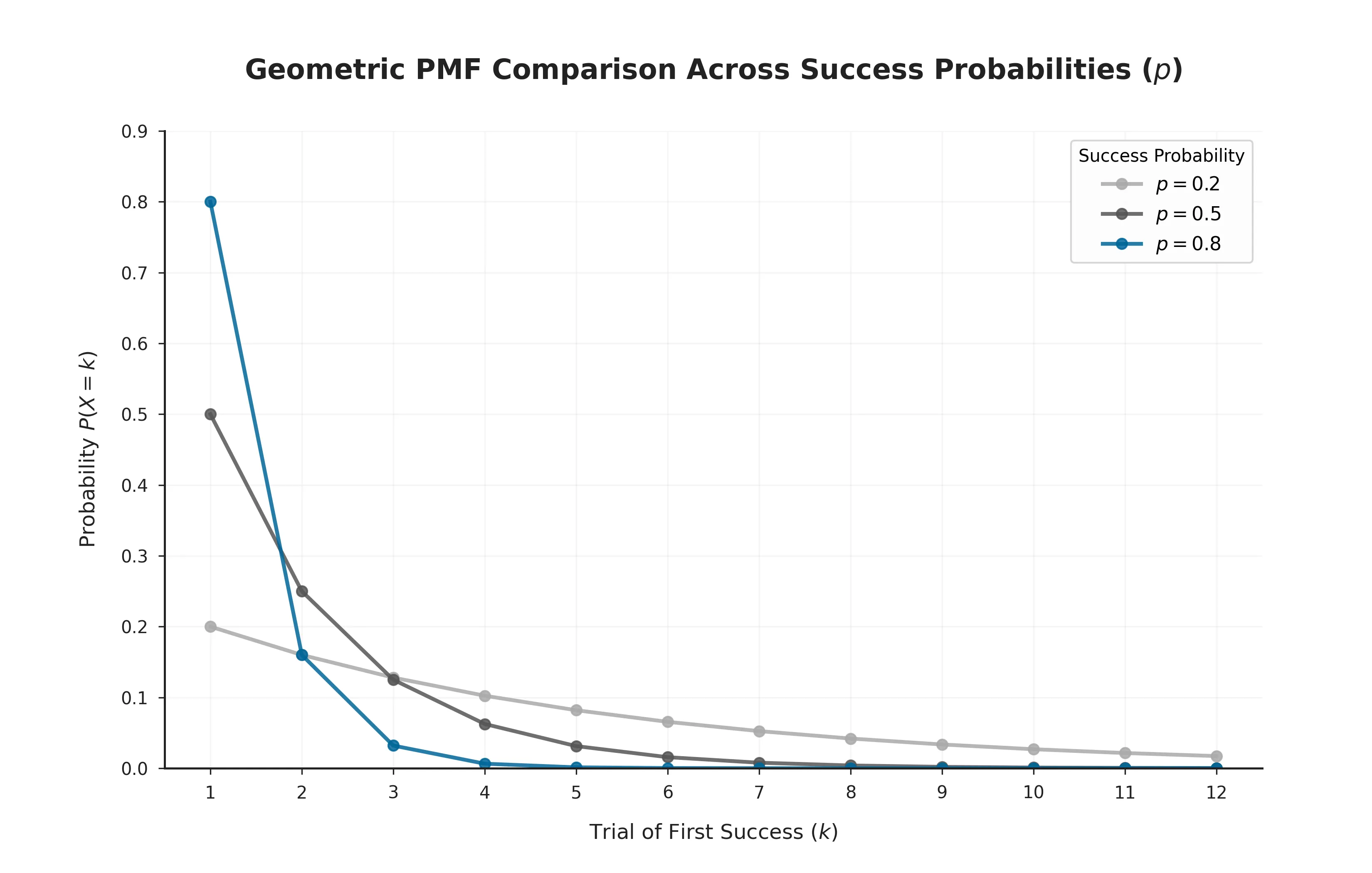
- Large \( p \) (close to 1) concentrates almost all probability mass at small values of \( k \), since success is likely on nearly every attempt and long runs of failure become increasingly rare.
- Small \( p \) (close to 0) spreads probability thinly across a long right tail: the mode remains fixed at \( k=1 \), but the mean \( 1/p \) and variance \( (1-p)/p^2 \) both grow large, so a typical outcome can be far from the most likely one.
- The PMF is strictly decreasing in \( k \) for every valid \( p \) - there is never a "hump" away from \( k=1 \), in contrast to the binomial distribution's shape, which can peak anywhere depending on \( n \) and \( p \).
- As \( p \to 0 \) with trials rescaled to continuous time, the geometric distribution converges to the exponential distribution, the natural continuous analogue of "waiting for the first event."
Moments & Generating Functions
The moment generating function (MGF) of a geometric random variable, valid for \( t < -\ln(1-p) \), is:
\[ M(t) = E\left[e^{tX}\right] = \frac{p\,e^{t}}{1-(1-p)e^{t}} \]Differentiating \( M(t) \) and evaluating at \( t=0 \) recovers the mean \( 1/p \) and, together with the second derivative, the variance \( (1-p)/p^2 \), matching the direct calculations in Core Properties.
The related probability generating function, more commonly used for discrete distributions, is:
\[ G(z) = E[z^X] = \frac{pz}{1-(1-p)z}, \qquad |z| < \frac{1}{1-p} \]and the characteristic function follows the same rational form, \( \varphi_X(t) = p\,e^{it} / \left[1-(1-p)e^{it}\right] \). The closed-form, rational-function shape of these generating functions is a hallmark of geometric series, echoing the geometric distribution's own origin as a sum of the terms \( (1-p)^{k-1}p \).
Cumulative Distribution Function
The cumulative distribution function (CDF), \( F(k) = P(X \le k) \), gives the probability that the first success occurs at or before the \( k \)-th trial. Unlike the binomial CDF, which has no simple closed form, the geometric CDF sums to a compact expression thanks to the geometric series:
\[ F(k) = P(X \le k) = 1-(1-p)^{k}, \qquad k = 1, 2, 3, \ldots \]This has an intuitive derivation of its own: the complementary event, \( X > k \), means the first \( k \) trials all failed, which happens with probability \( (1-p)^k \) by independence, so \( F(k) = 1 - P(X>k) = 1-(1-p)^k \). As with any discrete distribution, the geometric CDF is a staircase - here with infinitely many steps, one at each positive integer, each shrinking in height as \( k \) grows, and \( F(k) \to 1 \) as \( k \to \infty \).
Worked Example
Suppose the same online advertisement from the Bernoulli worked example is shown to a sequence of independent visitors, each clicking with probability \( p = 0.04 \) (a 4% click-through rate). Let \( X \sim \operatorname{Geometric}(0.04) \) denote the number of visitors shown the ad up to and including the one who first clicks. What are the mean and standard deviation of \( X \), and what is the probability that the first click happens on exactly the tenth visitor?
Step 1 - Mean: using \( E[X] = 1/p \) from Core Properties:
\[ E[X] = \frac{1}{0.04} = 25 \]Step 2 - Variance and standard deviation: using \( \operatorname{Var}(X) = (1-p)/p^2 \):
\[ \operatorname{Var}(X) = \frac{0.96}{0.04^2} = 600, \qquad \operatorname{SD}(X) = \sqrt{600} \approx 24.49 \]Step 3 - Probability the first click is on visitor 10: using the PMF with \( k=10 \):
\[ P(X=10) = (0.96)^{9}(0.04) \approx 0.6925 \times 0.04 \approx 0.0277 \]On average, the advertisement needs to be shown to 25 visitors before the first click arrives, with a fairly wide spread (standard deviation of roughly 24.5 visitors) reflecting the distribution's heavy right tail. There is roughly a 2.8% chance that the very first click happens on exactly the tenth visitor - a plausible but far from guaranteed early success, well short of the 25-visitor average.
Estimating p from Data
In practice, \( p \) is rarely known exactly and must be estimated from observed data. Given a single observation \( X = k \) (the first success occurred on the \( k \)-th trial), the maximum likelihood estimate (MLE) of \( p \) is:
\[ \hat{p} = \frac{1}{k} \]More usefully, given \( n \) independent geometric observations \( X_1, \ldots, X_n \), the MLE generalizes to the reciprocal of the sample mean, \( \hat{p} = n / \sum_{i=1}^{n} X_i \), which follows from the fact that \( E[X] = 1/p \) (see Core Properties) and matches the method-of-moments estimator exactly. This estimator is consistent - it converges to the true \( p \) as \( n \) grows - though, unlike the binomial proportion estimator, it is slightly biased upward for finite samples, a bias that shrinks as \( n \) increases.
Exponential Approximation
The geometric distribution is often described as the discrete-time analogue of the exponential distribution, and the connection becomes an explicit approximation when \( p \) is small.
When success is rare (\( p \) small) and trials occur at a fast, regular rate, the number of discrete trials until the first success, rescaled by \( p \), converges to a continuous exponential waiting time:
\[ pX \approx \operatorname{Exponential}(1), \qquad \text{equivalently} \qquad X \approx \operatorname{Exponential}(p) \]This mirrors the way the binomial distribution converges to the Poisson distribution as trials become frequent and individual success probability shrinks: both are instances of a discrete counting process converging to its continuous-time limit as the time step shrinks toward zero while the overall rate is held fixed. Both the geometric and exponential distributions share the memoryless property, which is exactly why this limiting relationship holds - memorylessness is preserved as the discrete trials are packed more and more densely into continuous time.
Generating Geometric Random Numbers
Because the geometric distribution's CDF has a simple closed form (see Cumulative Distribution Function), it can be generated directly by inverse transform sampling, without simulating individual Bernoulli trials one at a time:
- Draw \( U \sim \operatorname{Uniform}(0,1) \).
- Compute \( X = \left\lceil \dfrac{\ln(1-U)}{\ln(1-p)} \right\rceil \), the ceiling of that ratio of logarithms.
- Return \( X \) as the geometric draw.
This works by inverting the CDF \( F(k) = 1-(1-p)^k \) directly: solving \( U = F(k) \) for \( k \) and rounding up to the nearest integer produces a draw with exactly the right distribution, in a single step per sample rather than \( 1/p \) steps on average as a trial-by-trial simulation would require.
A simpler, if less efficient, alternative simulates trials directly: repeatedly draw \( U_i \sim \operatorname{Uniform}(0,1) \), treat the trial as a success once \( U_i < p \), and return the number of trials taken. This mirrors the Bernoulli-by-Bernoulli approach used to generate binomial variables, but runs, on average, \( 1/p \) iterations per draw rather than the single computation the inversion method needs.
In practice, these details are handled internally: for example, NumPy's numpy.random.geometric(p) and SciPy's scipy.stats.geom.rvs(p) both return draws from a Geometric\( (p) \) distribution without requiring the underlying inversion or trial-by-trial simulation to be implemented by hand.
A Short History
Like the binomial distribution, the geometric distribution's roots trace to the early study of repeated games of chance in the 17th and 18th centuries, where mathematicians analyzed the number of throws or draws needed before a particular outcome first appeared. Problems of exactly this form - "how many rolls of a die until the first six?" - appear in the correspondence and early treatises of probability pioneers studying dice games, well before the distribution was given a formal name or systematic treatment.
The distribution takes its name from the underlying geometric series, \( \sum_{k=1}^{\infty} (1-p)^{k-1}p = 1 \), a mathematical object studied since antiquity and formalized algebraically well before its probabilistic application. The systematic treatment of the geometric distribution as the discrete analogue of the exponential waiting-time distribution, and its recognition as the unique discrete distribution with the memoryless property, became a standard part of probability theory as the subject matured through the 19th and 20th centuries, alongside the broader development of discrete probability distributions as a unified family.
Where It Shows Up
Any scenario reducible to "how many independent yes/no attempts until the first success" is, in principle, geometric. A selection of concrete examples across statistics, computing, and engineering:
- Reliability testing - the number of manufacturing runs, or the number of stress-test cycles, until the first defect appears is commonly modeled as geometric.
- Networking and retransmission - the number of attempts a network protocol makes before a packet is successfully transmitted, under a fixed per-attempt success probability, is a standard geometric modeling exercise underlying retry-timeout analysis.
- Sales and marketing - the number of cold calls, or the number of ad impressions, needed before the first conversion is modeled as geometric, informing expected customer-acquisition cost.
- Genetics and screening - the number of individuals screened before the first carrier of a rare allele is found, under a fixed per-individual probability, follows a geometric distribution under simple independence assumptions.
- Queueing and service systems - the number of time slots a server waits before successfully transmitting, in slotted-ALOHA-style contention protocols, is modeled as geometric, underlying classic analyses of wireless channel access.
- Search and matching algorithms - the number of random probes needed before hitting an empty slot in open-addressing hash tables is analyzed using the geometric distribution, informing expected-time bounds for hashing schemes.
- Reinforcement learning - the number of exploratory attempts before an agent first discovers a rewarding action, under a fixed discovery probability per attempt, is a common geometric modeling simplification in analyzing exploration strategies.
- Games of chance - the number of rolls of a die until a particular face first appears, or the number of card draws until a particular suit is drawn (with replacement), are textbook geometric examples tracing back to the distribution's earliest historical use.
As with the Bernoulli distribution, the geometric model is occasionally misapplied when its two core assumptions - independence across trials and a constant success probability - are violated: if the chance of success changes with each attempt (for instance, sampling without replacement from a shrinking population), the negative hypergeometric distribution or other extensions are more appropriate than a plain geometric assumption (see Related Distributions).
Frequently Asked Questions
- It is the probability distribution of the number of independent trials needed to obtain the first success, where each trial has only two possible outcomes and the same success probability p.
- A Bernoulli distribution describes the outcome of a single trial with two possible outcomes. A geometric distribution describes how many such independent Bernoulli(p) trials must be repeated before the first success appears, so it is built from a sequence of Bernoulli trials rather than a single one.
- For a geometric random variable X counting trials until the first success, with success probability p, the mean is E[X] = 1/p and the variance is Var(X) = (1-p)/p^2.
- The geometric distribution is the only discrete distribution with the memoryless property: given that the first k trials have all failed, the probability distribution of the number of additional trials needed is identical to the distribution starting fresh, so past failures carry no information about the remaining wait.
- The geometric distribution counts trials needed to reach the first success, while the negative binomial distribution generalizes this to count trials needed to reach a fixed number r of successes; the geometric distribution is the special case of the negative binomial distribution with r = 1.
- Yes. One version counts the number of trials up to and including the first success, taking values 1, 2, 3, and so on. The other counts the number of failures before the first success, taking values 0, 1, 2, and so on. The two are related by a simple shift of one, but their formulas differ slightly, so it is important to check which convention a source is using.
- It is discrete: the random variable can take only whole-number values starting from 1 (or 0, depending on convention), so probability is described by a probability mass function rather than a probability density function.
- The Bernoulli distribution is the single-trial building block of every geometric trial, the negative binomial distribution generalizes the geometric distribution to counting trials until r successes, the exponential distribution is its continuous-time analogue and shares the memoryless property, and the Poisson distribution shares a close relationship with both through the theory of waiting times.