
Binomial Distribution
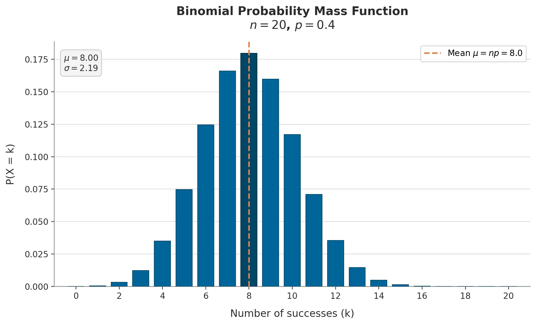
What Is a Binomial Distribution?
In probability theory and statistics, the binomial distribution is the discrete probability distribution of the number of successes in a fixed \( ' n ' \) number of independent trials, where each trial has only two possible outcomes - success or failure - and the same success probability \( p \) on every trial. It is the natural extension of the Bernoulli distribution from a single trial to many: flipping one coin is Bernoulli, counting the number of heads in ten flips of that same coin is binomial. See the formula below for the precise mathematical definition.
Each individual trial that makes up a binomial experiment is itself a Bernoulli trial, and the binomial distribution is formally defined as the sum of \( n \) independent, identically distributed Bernoulli\( (p) \) random variables. This makes it one of the most heavily used discrete distributions in applied statistics: any situation reducible to "how many out of \( n \) independent yes/no events came back yes" - the number of heads in repeated coin flips, the number of defective items in a batch, the number of visitors who convert on a landing page - is a candidate for a binomial model (see Where It Shows Up).
The Formula
The probability mass function (PMF) of a binomial distribution, which gives the probability of observing exactly \( k \) successes out of \( n \) independent trials, is:
\[ P(X = k) = \binom{n}{k} p^k (1-p)^{n-k}, \qquad k = 0, 1, 2, \ldots, n \]where \( \binom{n}{k} = \dfrac{n!}{k!(n-k)!} \) is the binomial coefficient, read "\( n \) choose \( k \)," which counts the number of distinct ways to arrange \( k \) successes among \( n \) trials, irrespective of order. The formula has a direct interpretation: \( p^k \) is the probability of any one specific sequence with exactly \( k \) successes, \( (1-p)^{n-k} \) is the probability that the remaining \( n-k \) trials are all failures, and the binomial coefficient accounts for every possible ordering of those \( k \) successes among the \( n \) trial positions.
Setting \( n=1 \) collapses the formula to \( P(X=k) = p^k(1-p)^{1-k} \) for \( k \in \{0,1\} \), exactly the Bernoulli PMF: the binomial distribution is the Bernoulli distribution's natural generalization from one trial to \( n \). Like the Bernoulli distribution and unlike the normal distribution's density, the binomial PMF assigns probability directly to a finite set of discrete outcomes, and the probabilities across all \( n+1 \) possible values of \( k \) sum to exactly \( 1 \).
Notation & Parameters
A binomial distribution with \( n \) trials and success probability \( p \) is written compactly as:
\[ X \sim \operatorname{Binomial}(n, p) \quad \text{or equivalently} \quad X \sim B(n, p) \]read as "\( X \) follows a binomial distribution with \( n \) trials and success probability \( p \)." Two parameters fully specify the distribution:
- \( n \) is the number of trials, a fixed positive integer, \( n \ge 1 \), known in advance of the experiment.
- \( p \) is the success probability on each individual trial, satisfying \( 0 \le p \le 1 \), and identical across all \( n \) trials.
- The support of the distribution - the set of values \( X \) can take - is the finite set of integers \( \{0, 1, 2, \ldots, n\} \), making the binomial distribution discrete, in contrast to continuous distributions such as the normal or uniform distributions.
- The two defining assumptions - independence across trials and an identical success probability \( p \) on every trial - are collectively referred to as the trials being i.i.d. (independent and identically distributed). Both assumptions matter: if trials influence one another, or if \( p \) itself drifts from trial to trial, the resulting count is no longer exactly binomial (see the Beta-binomial distribution for a common remedy).
Core Properties
The binomial distribution inherits its descriptive properties - mean, variance, skewness, kurtosis - directly from the fact that it is a sum of \( n \) independent Bernoulli variables, each contributing its own share to the total.
Mean (Expected Value)
The expected value of a binomial random variable follows directly from linearity of expectation applied to a sum of \( n \) Bernoulli\( (p) \) variables:
\[ E[X] = np \]Intuitively, if each of \( n \) trials succeeds with probability \( p \) on average, the expected total number of successes is simply \( n \) multiplied by \( p \). This identity is what allows \( p \) to be estimated directly from an observed count (see Estimating p from Data).
Variance
Because the \( n \) trials are independent, variances add directly, and the variance of a binomial random variable is \( n \) times the variance of a single Bernoulli trial:
\[ \operatorname{Var}(X) = np(1-p) \]For fixed \( n \), this quantity is maximized at \( p=0.5 \) - the same point where the underlying Bernoulli variance \( p(1-p) \) peaks - and shrinks toward \( 0 \) as \( p \) approaches either \( 0 \) or \( 1 \), where nearly every trial's outcome becomes predictable. The standard deviation is the square root of the variance, \( \operatorname{SD}(X) = \sqrt{np(1-p)} \).
Skewness
Skewness measures the asymmetry of a distribution. For a binomial distribution it is:
\[ \text{Skewness} = \frac{1-2p}{\sqrt{np(1-p)}} \]The numerator is identical to the Bernoulli skewness formula, but the extra factor of \( \sqrt{n} \) in the denominator means skewness shrinks toward \( 0 \) as \( n \) grows, for any fixed \( p \) strictly between \( 0 \) and \( 1 \). This is an early hint of the normal approximation: as more trials accumulate, the distribution becomes increasingly symmetric and bell-shaped, regardless of how skewed a single Bernoulli trial was.
Kurtosis
Kurtosis describes the shape of a distribution's tails relative to its center. For a binomial distribution, the excess kurtosis is:
\[ \text{Excess kurtosis} = \frac{1-6p(1-p)}{np(1-p)} \]As with skewness, the extra factor of \( n \) in the denominator drives excess kurtosis toward \( 0 \) as \( n \) grows large, matching the excess kurtosis of \( 0 \) that characterizes the normal distribution - another manifestation of the same underlying convergence.
Mode
The mode - the most probable count of successes - is given by \( \lfloor (n+1)p \rfloor \), the floor of \( (n+1)p \). When \( (n+1)p \) is itself an integer, both \( (n+1)p \) and \( (n+1)p - 1 \) are equally probable modes (a bimodal case), directly analogous to the bimodal case \( p=0.5 \) in the underlying Bernoulli distribution. As with the Bernoulli distribution, the mean \( np \) and mode generally do not coincide, though they draw closer together as \( n \) increases.
Shape as n and p Vary
The two parameters \( n \) and \( p \) control the shape of the binomial PMF in distinct, complementary ways, and seeing how the distribution deforms as each one changes builds useful intuition before moving to formal approximations.
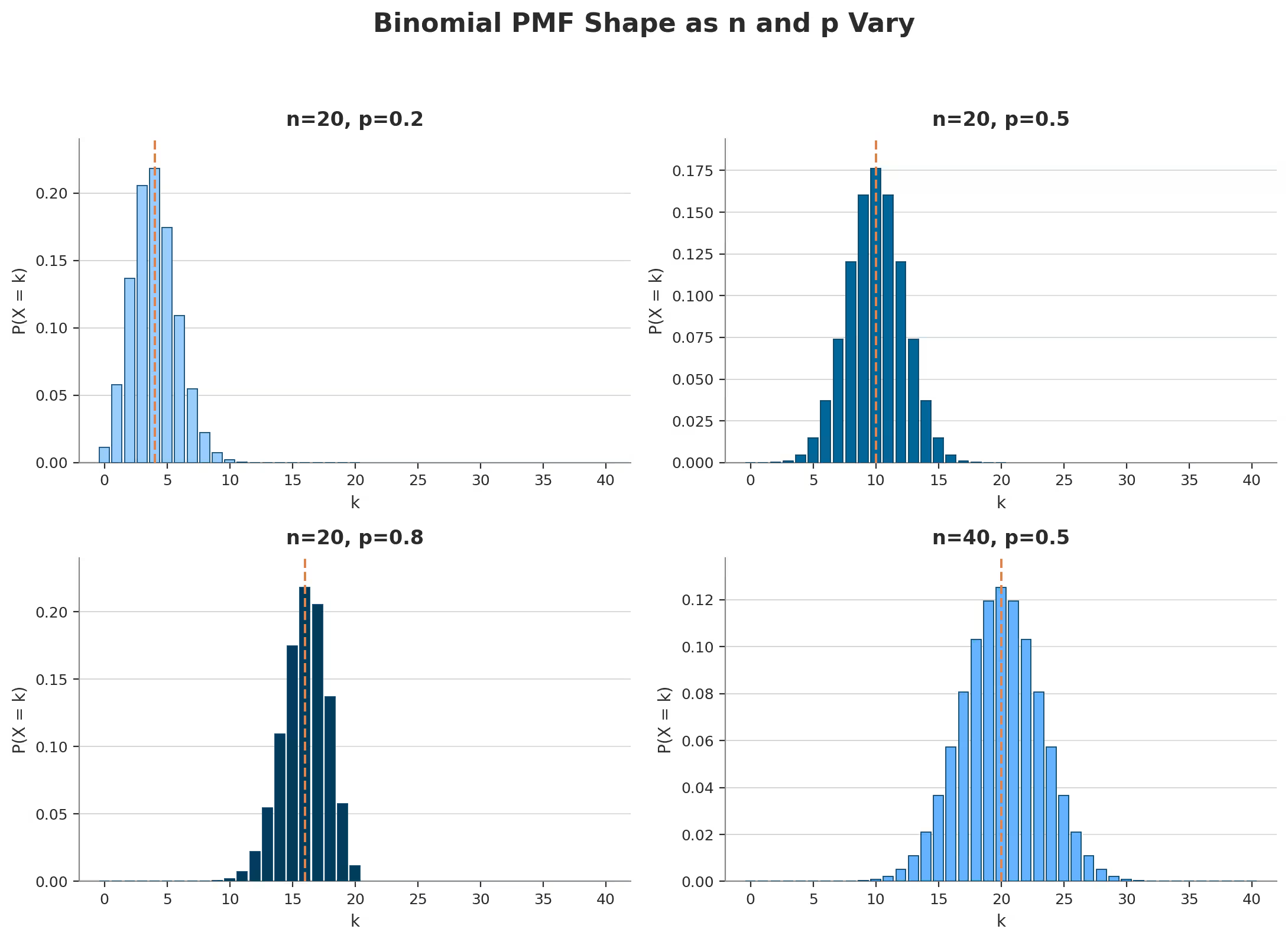
- Increasing \( n \) with \( p \) fixed spreads the distribution over a wider range of possible counts and, per the skewness and kurtosis formulas above, makes the shape progressively more symmetric and bell-like, consistent with the normal approximation.
- Moving \( p \) away from \( 0.5 \) with \( n \) fixed pulls the distribution's mass toward one end of its support (toward \( 0 \) for small \( p \), toward \( n \) for large \( p \)) and increases its skewness, mirroring the same asymmetry seen in the single-trial Bernoulli case.
- \( p = 0.5 \) is the unique point, for any \( n \), at which the distribution is perfectly symmetric, since \( P(X=k) = P(X=n-k) \) exactly when \( p = 1-p \).
- For small \( p \) and large \( n \) such that \( np \) stays moderate, the distribution develops a long right tail, and is well approximated by a Poisson distribution rather than a normal one.
Moments & Generating Functions
The moment generating function (MGF) of a binomial random variable follows directly from the MGF of a single Bernoulli trial, raised to the \( n \)-th power, since the MGF of a sum of independent variables is the product of their individual MGFs:
\[ M(t) = E\left[e^{tX}\right] = \left[(1-p) + p\,e^{t}\right]^n \]Differentiating \( M(t) \) and evaluating at \( t=0 \) recovers the mean \( np \) and, together with the second derivative, the variance \( np(1-p) \), matching the direct calculations in Core Properties.
The related probability generating function, more commonly used for discrete distributions, is similarly the \( n \)-th power of the Bernoulli probability generating function:
\[ G(z) = E[z^X] = \left[(1-p) + pz\right]^n \]and the characteristic function follows the same pattern, \( \varphi_X(t) = \left[(1-p) + p\,e^{it}\right]^n \). This "raise the single-trial function to the \( n \)-th power" pattern is a direct consequence of summing \( n \) independent, identically distributed variables, and reappears throughout the theory of sums of random variables.
Cumulative Distribution Function
The cumulative distribution function (CDF), \( F(k) = P(X \le k) \), gives the probability that a binomial variable takes a value at or below a given threshold. It is obtained by summing the PMF over all counts from \( 0 \) up to \( k \):
\[ F(k) = P(X \le k) = \sum_{i=0}^{\lfloor k \rfloor} \binom{n}{i} p^i (1-p)^{n-i} \]Unlike the Bernoulli distribution's simple three-step CDF, the binomial CDF is a staircase with up to \( n+1 \) distinct steps, one jump at each integer \( k \) in \( \{0, 1, \ldots, n\} \), each of height \( P(X=k) \). This staircase shape is characteristic of any discrete distribution's CDF, in contrast to the smooth S-curve of the normal distribution's CDF. In closed form, \( F(k) \) can also be written using the regularized incomplete beta function, \( F(k) = I_{1-p}(n-k, k+1) \), a relationship exploited by statistical software to evaluate binomial probabilities for large \( n \) without summing every term individually.
Worked Example
Suppose the same online advertisement from the Bernoulli worked example is shown independently to \( n = 20 \) visitors, each clicking with probability \( p = 0.04 \) (a 4% click-through rate). Let \( X \sim \operatorname{Binomial}(20, 0.04) \) denote the total number of clicks among these 20 visitors. What are the mean and standard deviation of \( X \), and what is the probability that exactly two visitors click?
Step 1 - Mean: using \( E[X] = np \) from Core Properties:
\[ E[X] = 20 \times 0.04 = 0.8 \]Step 2 - Variance and standard deviation: using \( \operatorname{Var}(X) = np(1-p) \):
\[ \operatorname{Var}(X) = 20 \times 0.04 \times 0.96 = 0.768, \qquad \operatorname{SD}(X) = \sqrt{0.768} \approx 0.876 \]Step 3 - Probability of exactly two clicks: using the PMF with \( k=2 \):
\[ P(X=2) = \binom{20}{2}(0.04)^2(0.96)^{18} = 190 \times 0.0016 \times 0.4796 \approx 0.1458 \]There is roughly a 14.6% chance that exactly two of the twenty visitors click the advertisement. Note how the expected count, \( 0.8 \), is itself not a possible outcome - the number of clicks must be a whole number - underscoring that the mean describes a long-run average across many independent batches of twenty visitors, not a prediction for any single batch.
Estimating p from Data
In practice, \( p \) is rarely known exactly and must be estimated from an observed count. Given a single observation \( X = k \) successes out of \( n \) known trials, the maximum likelihood estimate (MLE) of \( p \) is simply the observed proportion of successes:
\[ \hat{p} = \frac{k}{n} \]This is exactly the same estimator used for a Bernoulli sample (see Estimating p from Data on the Bernoulli page), which makes sense since a single binomial count of \( n \) trials carries the same information as \( n \) individual Bernoulli observations. The estimator is unbiased, since \( E[\hat p] = p \), and its variance, \( \operatorname{Var}(\hat p) = p(1-p)/n \), shrinks toward zero as \( n \) grows - the formal justification for why larger sample sizes give more reliable estimates of a success rate.
A common companion to the point estimate \( \hat p \) is a confidence interval for a proportion, most simply the Wald interval \( \hat p \pm z_{\alpha/2}\sqrt{\hat p(1-\hat p)/n} \), which relies on the normal approximation below and can behave poorly when \( n \) is small or \( \hat p \) is near \( 0 \) or \( 1 \); the Wilson and Clopper–Pearson intervals are more robust alternatives commonly used in practice.
Normal & Poisson Approximations
Computing exact binomial probabilities for large \( n \) can be cumbersome, so two well-known approximations are used depending on how \( n \) and \( p \) behave together.
Normal Approximation
When \( n \) is reasonably large and \( p \) is not too close to \( 0 \) or \( 1 \), the central limit theorem implies that a binomial random variable is approximately normally distributed with matching mean and variance:
\[ X \approx \mathcal{N}\big(np,\ np(1-p)\big) \]A widely used rule of thumb is that this approximation is reasonable once both \( np \ge 5 \) and \( n(1-p) \ge 5 \) (some sources require \( \ge 10 \) for greater accuracy), ensuring the distribution is not badly skewed toward either endpoint of its support. Because the binomial distribution is discrete and the normal distribution is continuous, a continuity correction of \( \pm 0.5 \) is often applied when using the normal approximation to estimate a discrete probability such as \( P(X \le k) \), improving accuracy for moderate \( n \).
Poisson Approximation
When \( n \) is large but \( p \) is small, such that the mean \( np \) stays moderate rather than growing without bound, the binomial distribution is instead well approximated by a Poisson distribution with rate \( \lambda = np \):
\[ X \approx \operatorname{Poisson}(\lambda), \qquad \lambda = np \]This is sometimes called the law of rare events, and is the formal justification for modeling counts of rare occurrences - typos on a page, radioactive decays in a fixed interval, server crashes in a day - as Poisson, since each is really the sum of a huge number of individually unlikely binomial trials. A common practical guideline favors the Poisson approximation over the normal one when \( n \ge 20 \) and \( p \le 0.05 \), or more generally whenever \( np \) is small while \( n \) itself is large.
Sums of Binomial Variables
The binomial distribution has a useful closure property, though a more restricted one than the normal distribution's closure under addition: if \( X_1 \sim \operatorname{Binomial}(n_1, p) \) and \( X_2 \sim \operatorname{Binomial}(n_2, p) \) are independent and share the same success probability \( p \), their sum is again binomial:
\[ X_1 + X_2 \sim \operatorname{Binomial}(n_1 + n_2,\ p) \]This follows immediately from viewing each binomial variable as a sum of Bernoulli\( (p) \) trials: adding \( X_1 \) and \( X_2 \) is the same as pooling \( n_1 + n_2 \) independent Bernoulli\( (p) \) trials into one larger count. The shared \( p \) is essential; if the two variables have different success probabilities, their sum is generally not binomial at all, and follows a more complex distribution instead.
Generating Binomial Random Numbers
Because a binomial variable is, by construction, a sum of \( n \) independent Bernoulli trials, the most direct way to generate one is to simulate all \( n \) trials individually and add up the successes:
- For each of \( i = 1, \ldots, n \), draw \( U_i \sim \operatorname{Uniform}(0,1) \) independently.
- Set \( X_i = 1 \) if \( U_i < p \), and \( X_i = 0 \) otherwise.
- Return \( X = \sum_{i=1}^{n} X_i \) as the binomial draw.
This direct simulation approach is simple but becomes computationally wasteful for very large \( n \), since it requires \( n \) separate uniform draws for a single binomial outcome. Statistical software libraries instead use faster algorithms - such as inversion of the CDF for small \( n \), or acceptance-rejection and transformation methods for large \( n \) - that avoid simulating every individual trial.
In practice, these details are handled internally: for example, NumPy's numpy.random.binomial(n, p) and SciPy's scipy.stats.binom.rvs(n, p) both return draws from a Binomial\( (n, p) \) distribution without requiring the underlying trial-by-trial simulation to be implemented by hand.
A Short History
The binomial distribution's roots trace to the same source as the Bernoulli distribution: Jacob Bernoulli's posthumously published 1713 work Ars Conjectandi ("The Art of Conjecturing"), where repeated trials with two outcomes were studied specifically to derive what is now called the binomial distribution, alongside an early form of the law of large numbers. The binomial coefficients themselves, arranged in Pascal's triangle, were known and studied centuries earlier across multiple mathematical traditions, well before their probabilistic interpretation was formalized.
In the following century, Abraham de Moivre showed in 1733 that the binomial distribution, for large \( n \), could be approximated by what is now recognized as the normal curve - an early version of what became the central limit theorem, and the historical origin of the normal approximation to the binomial described above. Later, Siméon Denis Poisson derived the complementary limit for rare events in 1837, giving the distribution that now bears his name and completing the pair of classical approximations still used today.
Where It Shows Up
Any scenario reducible to "count how many out of \( n \) independent yes/no trials succeeded" is, in principle, binomial. A selection of concrete examples across statistics, computing, and machine learning:
- Quality control - the number of defective items in a fixed-size sample drawn (with replacement, or from a very large batch) from a production run is modeled as binomial.
- A/B testing - the total number of visitors who convert out of a fixed number shown a given variant is a binomial count, with the two variants compared on their estimated success probabilities.
- Clinical trials - the number of patients who respond to a treatment out of a fixed number enrolled is commonly modeled as binomial, underlying hypothesis tests for treatment efficacy.
- Survey sampling - the number of respondents answering "yes" to a fixed-response survey question, out of a sample of \( n \) respondents, is modeled as binomial, the basis for margin of error calculations in polling.
- Genetics - the number of offspring inheriting a particular allele, out of a fixed number of offspring with known inheritance probability, follows a binomial distribution under simple Mendelian assumptions.
- Ensemble methods in machine learning - the number of individual classifiers in a voting ensemble that correctly predict a label can be modeled as binomial, informing analyses of why ensembles outperform single models when errors are sufficiently independent.
- Network reliability - the number of working components among \( n \) independent, identically reliable components in a system is a binomial count, used to compute overall system reliability.
- Sports and games analytics - the number of successful free throws out of a fixed number of attempts, or the number of wins in a fixed number of games against evenly matched opponents, is a standard binomial modeling exercise.
As with the Bernoulli distribution, the binomial model is occasionally misapplied when its two core assumptions - independence across trials and a constant success probability - are violated: clustered or correlated outcomes (patients treated at the same clinic, students in the same classroom) often call for extensions such as the Beta-binomial distribution or hierarchical models rather than a plain binomial assumption (see Related Distributions).
Frequently Asked Questions
- It is the probability distribution of the number of successes in a fixed number of independent trials, n, where each trial has only two possible outcomes and the same success probability p.
- A Bernoulli distribution describes the outcome of a single trial with two possible outcomes. A binomial distribution describes the total count of successes across n independent Bernoulli trials with the same success probability p; a Bernoulli distribution is the special case of a binomial distribution with n = 1.
- For a binomial random variable X with n trials and success probability p, the mean is E[X] = np and the variance is Var(X) = np(1 - p).
- A common rule of thumb is that the normal approximation is reasonable when both np and n(1 - p) are at least 5 (some sources use 10), so that the distribution is not too skewed toward either 0 or n.
- The binomial distribution counts successes in a fixed number of trials n with success probability p, while the Poisson distribution counts events over a continuous interval with an average rate lambda. The Poisson distribution arises as the limit of a binomial distribution as n grows large and p shrinks such that np stays fixed at lambda.
- The binomial coefficient, written as n choose k, equals n! divided by (k! times (n - k)!), and counts the number of distinct ways to choose k successes among n trials without regard to order.
- It is discrete: the random variable can take only whole-number values from 0 to n, so probability is described by a probability mass function rather than a probability density function.
- The Bernoulli distribution is the special case of the binomial distribution with n = 1, the sum of two independent binomial variables with the same p is itself binomial, the negative binomial distribution counts trials needed to reach a fixed number of successes, the Poisson distribution approximates it for large n and small p, and the normal distribution approximates it for large n via the central limit theorem.