Transformers in Machine Learning: Complete Guide to Transformer Architecture
Abstract
This article explains the Transformer architecture behind ChatGPT, Claude, Gemini, and other modern AI systems. Starting from the challenge of understanding sequences, it builds the model step by step through self-attention and the complete Transformer design. Along the way, key ideas are explained intuitively and reinforced with simple numerical examples.
1. The Sequence Problem
To understand why Transformers were invented, we must first understand the fundamental challenge they were designed to solve: how do we process sequences of information in a way that captures relationships between distant elements?
Consider the English sentence: "The bank executive was convicted because she had embezzled funds from the bank." Most humans understand instantly that the two instances of "bank" refer to the same entity-a financial institution. Yet for a neural network, this is not trivial. The word "bank" at position 2 and the word "bank" at position 16 are separated by 14 tokens. If your neural network can only "see" a fixed window of context, it may miss this relationship entirely. If your network processes tokens sequentially, one at a time, it must maintain the relevance of early information across a long sequence-a task at which recurrent networks famously struggle due to the vanishing gradient problem.
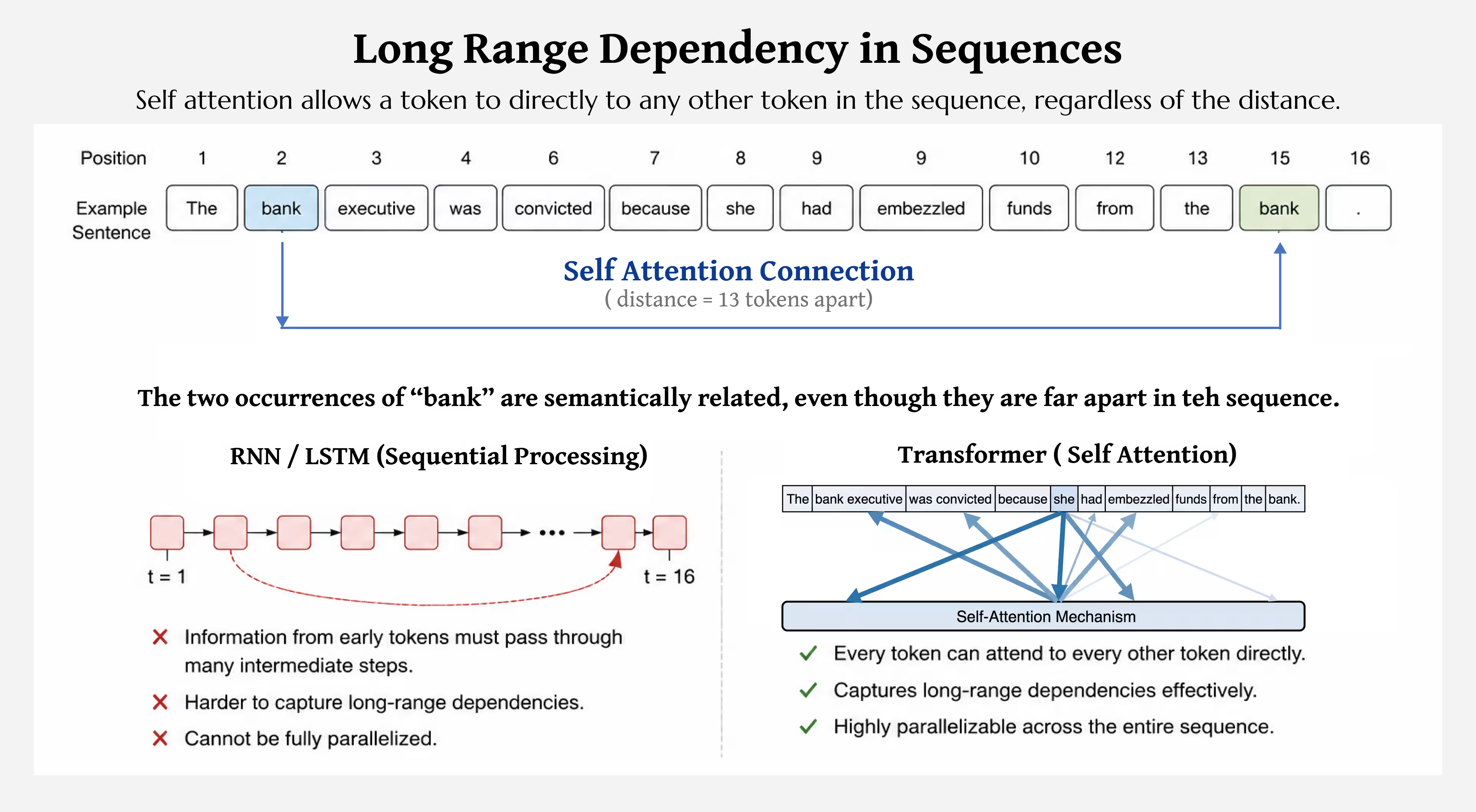
This is the core problem: how do we allow a neural network to attend to any part of a sequence, regardless of distance, while capturing the relationships between all pairs of tokens?
Throughout the 2000s and 2010s, neural language processing was dominated by recurrent neural networks (RNNs) and their variants-long short-term memory networks (LSTMs) and gated recurrent units (GRUs). These architectures process sequences one token at a time, maintaining a hidden state that is updated at each step. The advantage is simplicity: the hidden state provides a bottleneck through which information must pass, and the recurrent structure naturally captures sequential information.
But this sequential processing has a critical weakness. Because tokens are processed one at a time, information from early tokens must be compressed into the hidden state and passed through many layers of gates and nonlinearities. By the time we reach token \( t = 100 \), the information from token \( t = 1 \) has been through a hundred steps of transformation. Each step is a potential opportunity for information to degrade, dilute, or disappear entirely. This is the vanishing gradient problem: when gradients are backpropagated through many sequential steps, they become exponentially smaller, making it difficult for the network to learn long-range dependencies.
LSTMs and GRUs were designed to mitigate this problem through gating mechanisms-learnable pathways that decide what information to preserve and what to discard. These architectures were transformative and enabled significant progress. Yet they still process sequences sequentially, which introduces a fundamental computational bottleneck: you cannot parallelize the computation across the sequence. If you want to process a sequence of length \( T \), you must wait for step 1 to complete before computing step 2, and so on. For large language models trained on enormous datasets, this sequential constraint is a severe limitation.
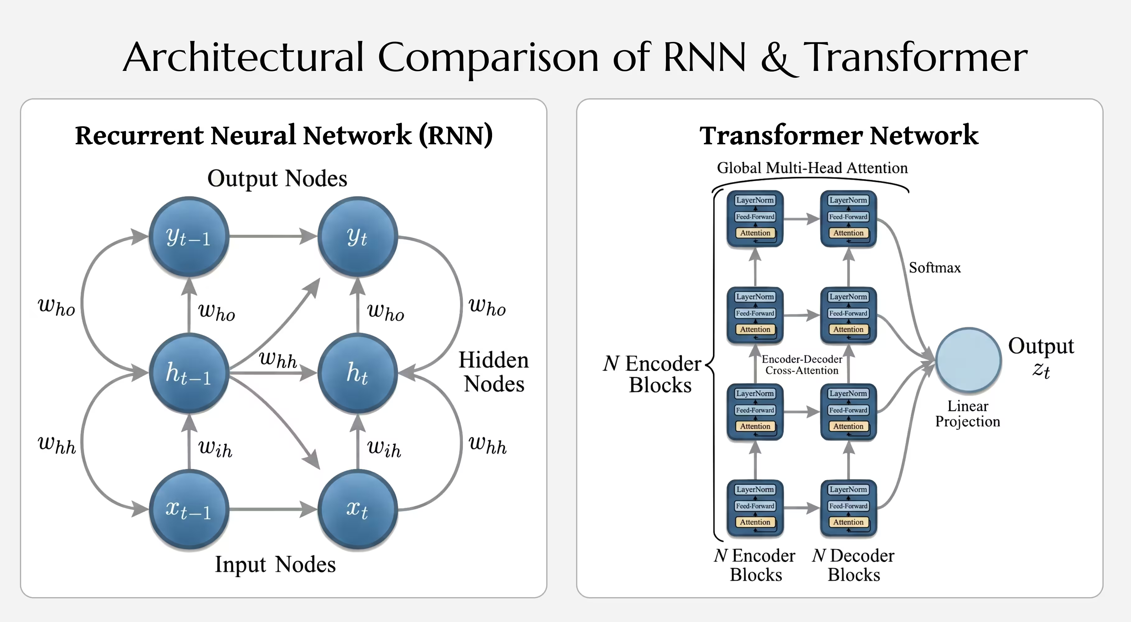
The Transformer breaks this constraint. It introduces a mechanism called self-attention that allows every token in a sequence to attend directly to every other token, simultaneously, and in parallel. The distance between tokens becomes irrelevant-a token at position 1 can attend to a token at position 1000 with the same computational cost as attending to an adjacent token. Moreover, because all tokens are processed in parallel, the entire sequence can be computed simultaneously on modern hardware (GPUs and TPUs), resulting in dramatic speedups during training.
The cost of this capability is a quadratic increase in memory and computation: for a sequence of length \( T \), the self-attention mechanism requires \( O(T^2) \) comparisons. For long sequences, this becomes expensive. But for the sequences encountered in language modeling-typically measured in hundreds or low thousands of tokens-this cost is tractable and vastly outweighed by the benefits of parallelization and superior learning of long-range dependencies.
2. A Brief History of Attention
Self-attention did not emerge from nowhere. It was the culmination of years of research into attention mechanisms, beginning in the context of machine translation with recurrent sequence-to-sequence models.
In the early 2010s, the standard approach to machine translation was the sequence-to-sequence (seq2seq) architecture: an encoder RNN would process the source language sentence and compress it into a fixed-size vector, which would then be passed to a decoder RNN to generate the target language sentence. This architecture worked surprisingly well, but it had an obvious weakness: the entire meaning of a sentence, potentially dozens of words long, had to be compressed into a single fixed-size vector. As sentence length increased, performance degraded rapidly.
In 2014, Bahdanau, Cho, and Bengio introduced the attention mechanism for seq2seq models. The key insight was simple: instead of compressing the entire source sentence into a single vector, why not allow the decoder to "attend to" different parts of the source sentence at each decoding step? Specifically, when generating the next target word, the decoder could compute a weighted sum of all encoder hidden states, where the weights were learned to focus on the parts of the source sentence most relevant to the current decoding step.
This was a major breakthrough. It allowed models to learn alignments between source and target languages automatically, without explicit annotation. Models trained with attention achieved state-of-the-art results on machine translation and became the standard architecture.
However, the original attention mechanism still required an RNN as the encoder and decoder. Tokens were still processed sequentially. The RNN was necessary to capture sequential information and to provide the hidden states that attention could operate on. This remained a computational bottleneck.
In 2017, the authors of "Attention Is All You Need" asked a radical question: if attention is so powerful, why do we need the RNN at all? Could we build an architecture that uses only attention mechanisms, dispensing with recurrence entirely? The answer was yes-and the result was the Transformer.
The insight was that by combining attention with positional encoding (a way to encode the position of each token in the sequence) and stacking multiple layers of attention, you could capture both long-range dependencies and sequential information, all while maintaining the ability to process the entire sequence in parallel. This was a fundamental shift in how neural networks approached sequence modeling.
3. Self-Attention from First Principles
3.1 The Problem: Relating Tokens to Tokens
The core operation of a Transformer is self-attention. Let's build it from scratch, starting with the simplest possible motivation.
Suppose we have a sequence of tokens: "The quick brown fox jumps." Each token is represented as a vector. Let's denote the embedding of token \( i \) as \( \mathbf{x}_i \in \mathbb{R}^{d} \), where \( d \) is the dimension of the embedding (e.g., \( d = 512 \)). For a sequence of \( n \) tokens, we can stack these embeddings into a matrix:
\[ \mathbf{X} = \begin{bmatrix} \mathbf{x}_1 \\ \mathbf{x}_2 \\ \vdots \\ \mathbf{x}_n \end{bmatrix} \in \mathbb{R}^{n \times d} \]Each row is one token's embedding. Now, the question: how do we compute a new representation of each token that incorporates information from other tokens in the sequence?
A naive approach would be to average all the embeddings. This would give us a single vector that represents the entire sequence. But this loses positional information-it treats all tokens equally. We need something more sophisticated: a mechanism that computes, for each token, a weighted average of all tokens, where the weights depend on the semantic relationship between tokens.
Here's the intuition: if we're processing the word "fox," we should pay more attention to words like "quick" and "brown" (which are likely adjectives describing the fox) and less attention to words like "the" or "jumps" (which serve other grammatical roles). The weights should be learned by the model, not fixed by hand.
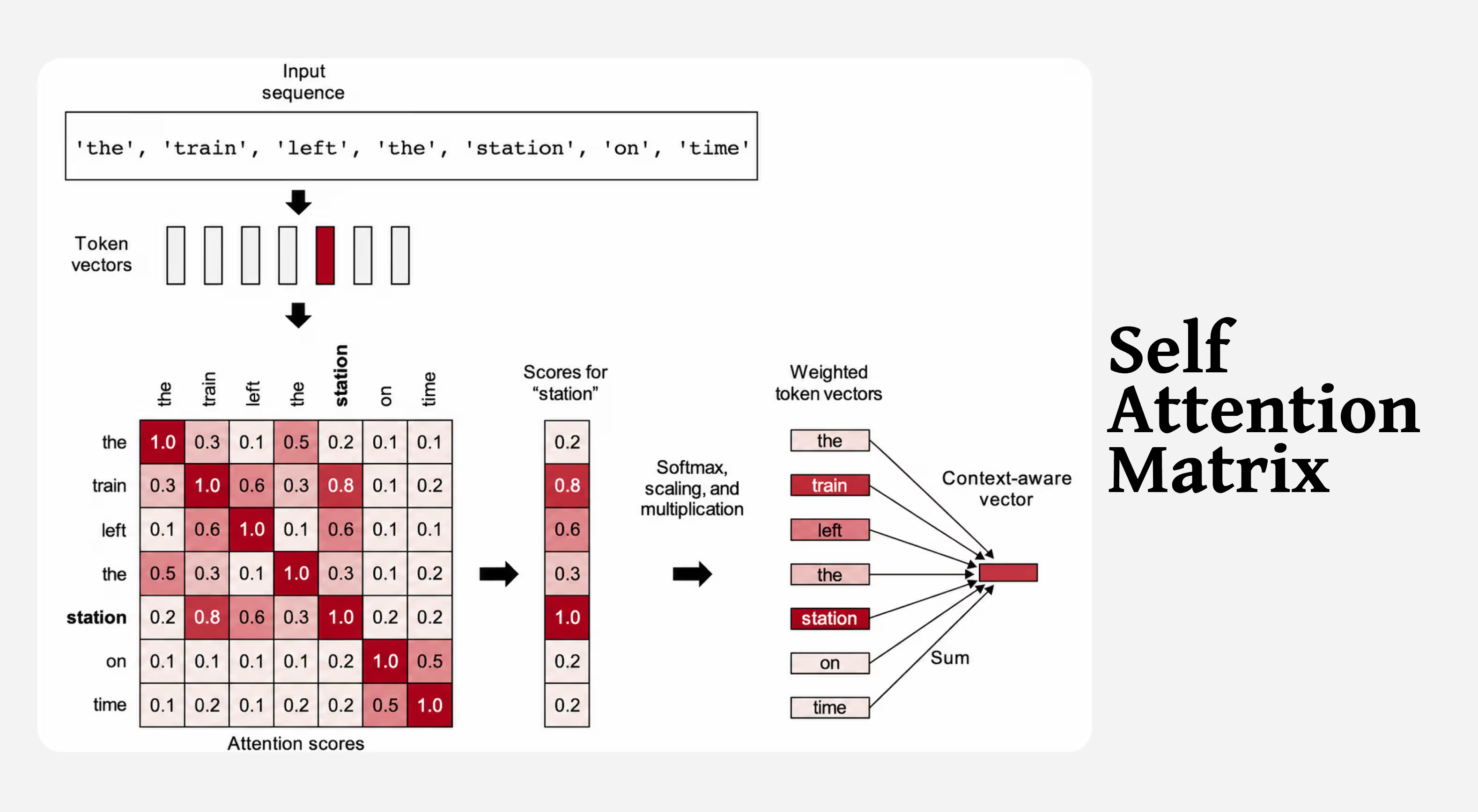
Self-attention achieves this by learning three projections of each token: a query, a key, and a value.
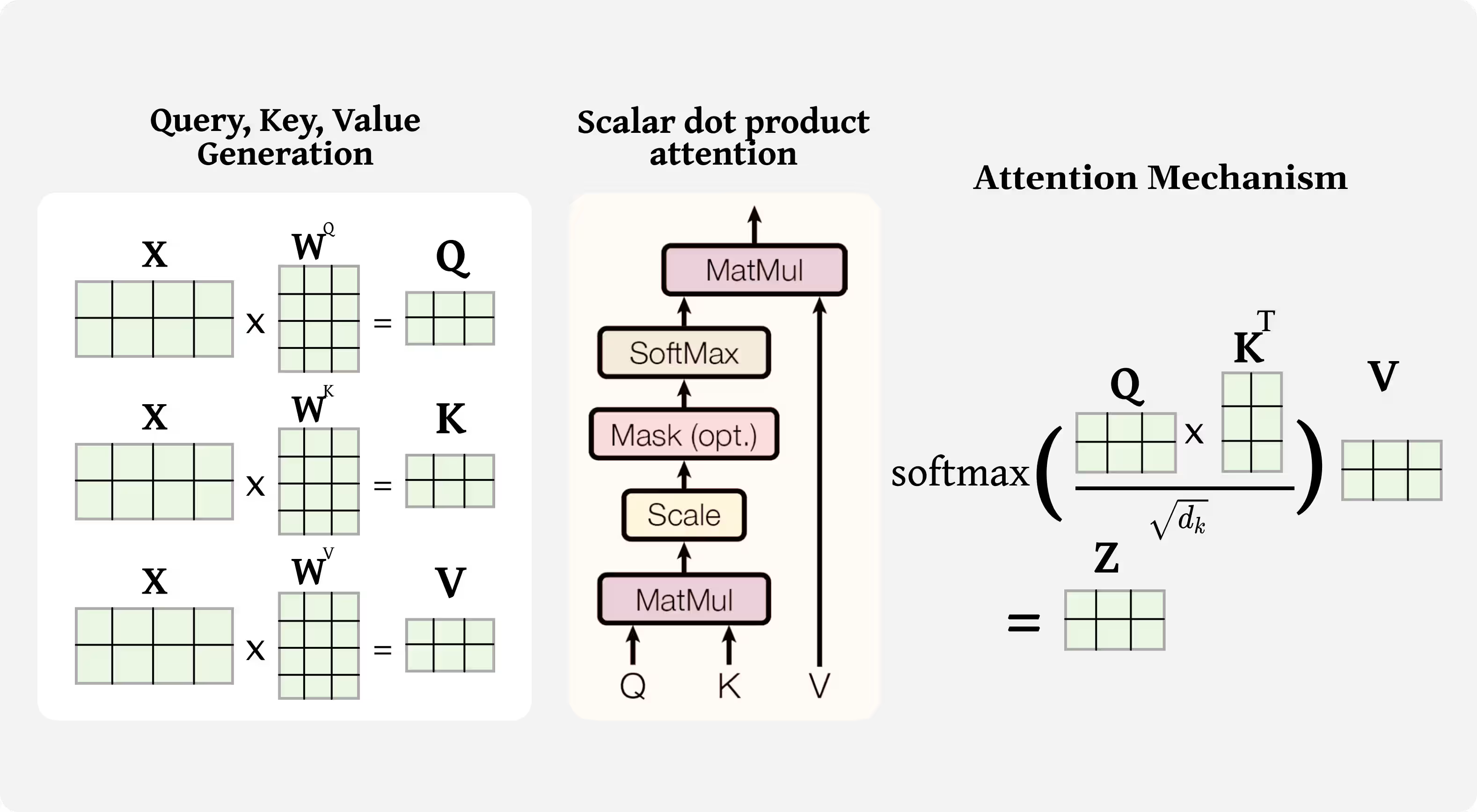
QKT/√dk, which are normalized with the softmax function and used to aggregate value vectors into contextualized token representations. 3.2 Queries, Keys, and Values
For each token embedding \( \mathbf{x}_i \), we compute three vectors:
\[ \mathbf{q}_i = \mathbf{W}^Q \mathbf{x}_i \quad \text{(query)} \] \[ \mathbf{k}_i = \mathbf{W}^K \mathbf{x}_i \quad \text{(key)} \] \[ \mathbf{v}_i = \mathbf{W}^V \mathbf{x}_i \quad \text{(value)} \]where \( \mathbf{W}^Q, \mathbf{W}^K, \mathbf{W}^V \in \mathbb{R}^{d \times d} \) are learned projection matrices. These matrices are the same for all tokens in a given attention layer-they are shared parameters.
What do these mean intuitively? Think of the query as a question: "What information from other tokens is relevant to me?" The keys are like tags on other tokens: "I contain this type of information." The values are the actual information being computed: "If you attend to me, here's what you get."
To make this concrete with a worked example: suppose token 3 is the word "fox." Its query vector \( \mathbf{q}_3 \) is asking "What tokens are relevant to my processing?" When we compare \( \mathbf{q}_3 \) to the key of token 2 ("brown"), if the dot product is large, it means token 2 is relevant to token 3. If we then attend to token 2, we receive its value vector \( \mathbf{v}_2 \), which contains its learned semantic information.
3.3 Computing Attention Weights
Now we need to compute how much each token should attend to each other token. We do this by comparing queries to keys using a dot product. For token \( i \), the dot product between its query and the key of token \( j \) is:
\[ \text{score}_{ij} = \mathbf{q}_i \cdot \mathbf{k}_j \]A large dot product means the query and key are aligned, suggesting token \( j \) is relevant to token \( i \). A small or negative dot product suggests low relevance. But these raw scores can have very different magnitudes depending on the dimension \( d \) of the embedding. To stabilize this, we scale by \( \sqrt{d} \):
\[ \text{score}_{ij} = \frac{\mathbf{q}_i \cdot \mathbf{k}_j}{\sqrt{d}} \]This scaling is crucial. Without it, the dot products can grow very large (since \( d \) is typically 512 or more), which can cause the softmax in the next step to become saturated, with gradients too small to learn effectively.
Now we convert these scores to weights using the softmax function, which ensures they sum to 1 and are all positive:
\[ \alpha_{ij} = \text{softmax}_j\left(\frac{\mathbf{q}_i \cdot \mathbf{k}_j}{\sqrt{d}}\right) = \frac{\exp\left(\frac{\mathbf{q}_i \cdot \mathbf{k}_j}{\sqrt{d}}\right)}{\sum_{k=1}^{n} \exp\left(\frac{\mathbf{q}_i \cdot \mathbf{k}_j}{\sqrt{d}}\right)} \]The softmax is applied across all tokens \( j = 1, \ldots, n \). For each query \( i \), we get a probability distribution \( [\alpha_{i1}, \alpha_{i2}, \ldots, \alpha_{in}] \) over all tokens. If \( \alpha_{i2} \) is 0.6, it means token \( i \) will pay 60% attention to token 2.
3.4 Aggregating Values
Finally, we compute a weighted average of all value vectors using the attention weights:
\[ \text{output}_i = \sum_{j=1}^{n} \alpha_{ij} \mathbf{v}_j \]This output is a new representation of token \( i \) that incorporates information from all other tokens in the sequence, weighted by attention.
3.5 Worked Example: Hand Calculation
Let's work through a concrete example. Suppose we have a 2-token sequence with embeddings of dimension \( d = 2 \):
\[ \mathbf{x}_1 = \begin{bmatrix} 1 \\ 0 \end{bmatrix}, \quad \mathbf{x}_2 = \begin{bmatrix} 0 \\ 1 \end{bmatrix} \]And suppose our projection matrices are (for simplicity):
\[ \mathbf{W}^Q = \begin{bmatrix} 1 & 0 \\ 0 & 1 \end{bmatrix}, \quad \mathbf{W}^K = \begin{bmatrix} 1 & 0 \\ 0 & 1 \end{bmatrix}, \quad \mathbf{W}^V = \begin{bmatrix} 0.5 & 0.5 \\ 0.5 & 0.5 \end{bmatrix} \]Computing queries, keys, and values:
\[ \mathbf{q}_1 = \begin{bmatrix} 1 \\ 0 \end{bmatrix}, \quad \mathbf{k}_1 = \begin{bmatrix} 1 \\ 0 \end{bmatrix}, \quad \mathbf{v}_1 = \begin{bmatrix} 0.5 \\ 0.5 \end{bmatrix} \] \[ \mathbf{q}_2 = \begin{bmatrix} 0 \\ 1 \end{bmatrix}, \quad \mathbf{k}_2 = \begin{bmatrix} 0 \\ 1 \end{bmatrix}, \quad \mathbf{v}_2 = \begin{bmatrix} 0.5 \\ 0.5 \end{bmatrix} \]Now we compute the attention scores for token 1:
\[ \text{score}_{11} = \frac{\mathbf{q}_1 \cdot \mathbf{k}_1}{\sqrt{2}} = \frac{1 \cdot 1 + 0 \cdot 0}{\sqrt{2}} = \frac{1}{\sqrt{2}} \approx 0.707 \] \[ \text{score}_{12} = \frac{\mathbf{q}_1 \cdot \mathbf{k}_2}{\sqrt{2}} = \frac{1 \cdot 0 + 0 \cdot 1}{\sqrt{2}} = 0 \]Applying softmax:
\[ \alpha_{11} = \frac{\exp(0.707)}{\exp(0.707) + \exp(0)} = \frac{2.028}{2.028 + 1} \approx 0.67 \] \[ \alpha_{12} = \frac{\exp(0)}{\exp(0.707) + \exp(0)} = \frac{1}{3.028} \approx 0.33 \]And the output for token 1:
\[ \text{output}_1 = 0.67 \begin{bmatrix} 0.5 \\ 0.5 \end{bmatrix} + 0.33 \begin{bmatrix} 0.5 \\ 0.5 \end{bmatrix} = \begin{bmatrix} 0.5 \\ 0.5 \end{bmatrix} \]Interestingly, in this case, the output for token 1 is the same regardless of the attention weights because both value vectors are identical. This illustrates an important point: the attention mechanism is only as useful as the values it's aggregating. If all values are the same, attention is meaningless. In practice, the projection matrices \( \mathbf{W}^V \) are learned such that tokens produce distinct value vectors.
3.6 Matrix Formulation
In practice, we compute attention for all tokens simultaneously using matrix operations. Define:
\[ \mathbf{Q} = \mathbf{X} \mathbf{W}^Q, \quad \mathbf{K} = \mathbf{X} \mathbf{W}^K, \quad \mathbf{V} = \mathbf{X} \mathbf{W}^V \]Then the attention operation can be written compactly as:
\[ \boxed{\text{Attention}(\mathbf{Q}, \mathbf{K}, \mathbf{V}) = \text{softmax}\left(\frac{\mathbf{Q} \mathbf{K}^T}{\sqrt{d}}\right) \mathbf{V}} \]This is the fundamental equation of self-attention. Let's parse it:
\( \mathbf{Q} \mathbf{K}^T \) is an \( n \times n \) matrix where element \( (i, j) \) is the dot product \( \mathbf{q}_i \cdot \mathbf{k}_j \)-the similarity between query \( i \) and key \( j \). Dividing by \( \sqrt{d} \) scales these similarities. Softmax is applied row-wise, converting each row into a probability distribution. Finally, multiplying by \( \mathbf{V} \) aggregates the value vectors according to these probabilities.
The result is an \( n \times d \) matrix where row \( i \) is the output representation of token \( i \), incorporating information from all tokens in the sequence.
3.6b PyTorch Implementation
The matrix formulation maps directly to code. Here is a minimal, readable scaled dot-product attention in PyTorch:
import torch
import torch.nn.functional as F

def scaled_dot_product_attention(Q, K, V, mask=None):
    """
    Args:
        Q: (batch, heads, seq_len, d_k)
        K: (batch, heads, seq_len, d_k)
        V: (batch, heads, seq_len, d_k)
        mask: optional causal or padding mask
    Returns:
        output: (batch, heads, seq_len, d_k)
        weights: (batch, heads, seq_len, seq_len)
    """
    d_k = Q.size(-1)

    # Compute raw attention scores
    scores = torch.matmul(Q, K.transpose(-2, -1)) / d_k ** 0.5  # (B, H, T, T)

    # Apply causal/padding mask (optional)
    if mask is not None:
        scores = scores.masked_fill(mask == 0, float('-inf'))

    # Softmax → attention weights
    weights = F.softmax(scores, dim=-1)  # rows sum to 1

    # Weighted sum of values
    output = torch.matmul(weights, V)    # (B, H, T, d_k)
    return output, weights

    if __name__ == "__main__":
    B, H, T, d_k = 2, 8, 64, 64# batch=2, 8 heads, seq=64, dim=64
    Q = torch.randn(B, H, T, d_k)
    K = torch.randn(B, H, T, d_k)
    V = torch.randn(B, H, T, d_k)

    out, w = scaled_dot_product_attention(Q, K, V)
    print(f"Output shape : {out.shape}")   # → torch.Size([2, 8, 64, 64])
    print(f"Weights sum  : {w[0,0,0].sum():.4f}")  # → 1.0000
Three things to notice: the scaling by d_k ** 0.5 happens before softmax; the mask is applied by setting positions to -inf so softmax drives them to zero; and the final output is identical in shape to the input queries.
3.7 Why This Works: The Geometry of Dot Products
The use of dot products for computing attention weights is not arbitrary. The dot product has a natural geometric interpretation: it measures the alignment between two vectors. If two vectors point in the same direction, their dot product is large and positive. If they point in opposite directions, it's large and negative. If they're orthogonal, it's zero.
By using dot products to compare queries and keys, we're asking: "In which direction does the query point? Which keys point in similar directions?" This is a natural notion of semantic relevance. Two tokens whose embeddings have learned to align in high-dimensional space are likely to be semantically related.
The reason we scale by \( \sqrt{d} \) is subtle. When \( d \) is large (say, 512), vectors are generally nearly orthogonal to each other (this is a property of high-dimensional geometry). The dot product of two random vectors of dimension \( d \) has standard deviation \( \sqrt{d} \). If we don't scale by \( \sqrt{d} \), the softmax will receive very small or very large inputs, leading to either uniform attention or overly peaked attention. Scaling by \( \sqrt{d} \) ensures the input to softmax has reasonable variance.
4. Positional Information
4.1 The Problem: Permutation Invariance
The self-attention mechanism, as described so far, has a significant limitation: it is permutation invariant. If you shuffle the order of tokens in the input sequence, the output-before any positional information is added-would remain the same. The query-key comparisons depend only on the semantic content of the tokens, not their positions.
But the order of tokens is crucial for meaning. "John loves Mary" and "Mary loves John" have very different meanings, yet their token embeddings are identical, just in a different order. An attention mechanism that ignores position would treat these sentences as equivalent, which is clearly wrong.
How do we incorporate positional information? There are several approaches. The naive approach would be to concatenate a one-hot vector indicating the position to each token embedding. But this has problems: it doesn't generalize to longer sequences, and the "position" feature doesn't interact meaningfully with the semantic content of the token.
The original Transformer paper proposed a more elegant solution: encode position using sinusoidal functions. The intuition is that sinusoidal functions have properties that make them ideal for this purpose: they are smooth, periodic, and bounded, allowing the model to learn both absolute and relative position easily.
4.2 Sinusoidal Positional Encoding
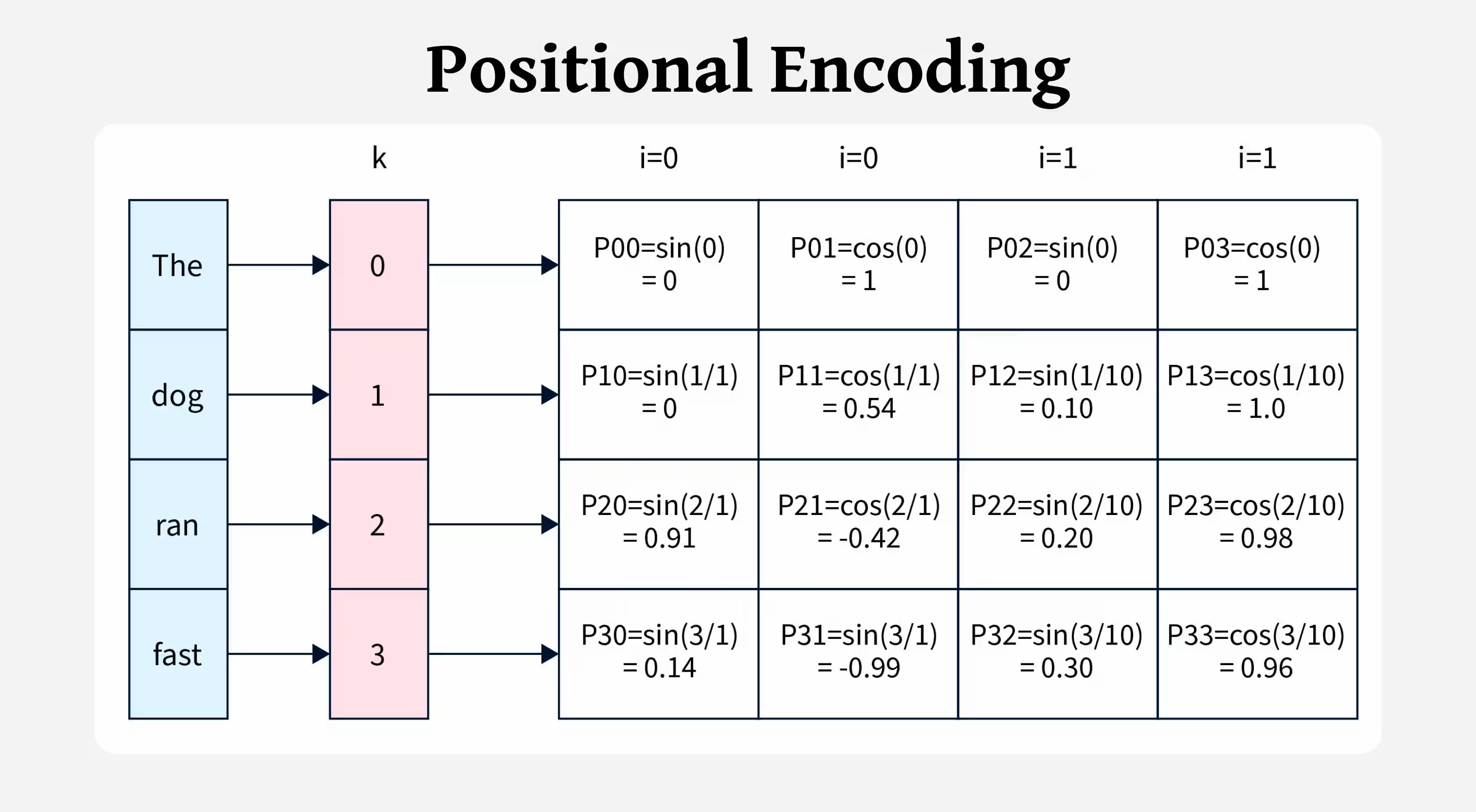
For token position \( \text{pos} \) (starting from 0) and dimension \( i \) (of the embedding), the positional encoding is:
\[ \text{PE}(\text{pos}, 2i) = \sin\left(\frac{\text{pos}}{10000^{2i/d}}\right) \] \[ \text{PE}(\text{pos}, 2i+1) = \cos\left(\frac{\text{pos}}{10000^{2i/d}}\right) \]In other words, we use sine for even dimensions and cosine for odd dimensions. Each dimension oscillates at a different frequency, determined by the base 10000 and the dimension index \( i \).
Let's build intuition. For dimension 0 (\( i = 0 \)), the frequency is \( 1 / 10000^0 = 1 \), so \( \text{PE}(\text{pos}, 0) = \sin(\text{pos}) \). This completes a full cycle every \( 2\pi \approx 6.28 \) positions. For dimension 2 (\( i = 1 \)), the frequency is \( 1 / 10000^{2/d} \), which is much smaller, so the sinusoid oscillates more slowly. As we move to higher dimensions, the frequencies decrease exponentially, creating a logarithmic distribution of frequencies.
Why is this clever? Consider two positions \( \text{pos} \) and \( \text{pos} + k \). The difference in their positional encodings encodes information about the relative distance \( k \). Because we use sinusoids of different frequencies, the model can learn both fine-grained relative positions (using high-frequency components) and coarse-grained structure (using low-frequency components).
Here's a worked example. Suppose \( d = 4 \) and we want the positional encodings for positions 0 and 1:
\[ \text{PE}(0, :) = [\sin(0), \cos(0), \sin(0), \cos(0)] = [0, 1, 0, 1] \] \[ \text{PE}(1, :) = [\sin(1), \cos(1), \sin(1 / 100), \cos(1 / 100)] \approx [0.841, 0.540, 0.01, 1.0] \]Each position has a unique encoding (or nearly unique-in practice, sequences rarely exceed 10,000 tokens, and the encodings are unique enough for the model to distinguish positions).
4.3 Adding Positional Encodings to Embeddings
The final step is simple: add the positional encoding to the token embedding:
\[ \mathbf{x}'_i = \mathbf{x}_i + \text{PE}(\text{pos}, :) \]This modified embedding now contains both semantic information (from the original \( \mathbf{x}_i \)) and positional information (from \( \text{PE} \)). The self-attention mechanism operates on these enriched embeddings, allowing it to consider both what tokens are and where they are.
4.4 Why Sinusoids? Alternatives and Intuitions
One might ask: why not learn the positional encodings as parameters? This would certainly be flexible. In fact, some models (like BERT) do use learned position embeddings. The advantage of sinusoidal encoding is generalization: it allows the model to handle sequences longer than any it saw during training. If you trained on sequences of length 512 with learned position embeddings, the model wouldn't know how to handle a sequence of length 1024-the position embeddings would be outside the training distribution.
Sinusoidal encodings, by contrast, are defined for any position, so a model trained with them can generalize to arbitrarily long sequences (though performance may degrade for positions far outside the training distribution).
Another advantage: sinusoidal encodings have a mathematical property that makes relative positions learnable. A recent position \( (pos + k) \) can be expressed as a linear transformation of position \( pos \) via rotation matrices, meaning the model can learn relationships like "the token 5 positions ahead" without seeing that exact offset during training.
5. Multi-Head Attention
5.1 Motivation: Parallel Representations
The self-attention mechanism computes a weighted average of values using a single set of query-key-value projections. But there's no reason to limit ourselves to a single representation. Different aspects of the relationship between tokens might be captured by different projections.
Consider the sentence "The animal didn't cross the street because it was too tired." The word "it" is ambiguous-does it refer to "the animal" or "the street"? A human reader understands that pronouns typically refer to the nearest noun phrase that matches the gender and number, so "it" refers to "the animal." But capturing this requires a syntactic understanding of noun phrases and agreement patterns.
Now consider "The animal didn't cross the street because it was too crowded." Here, "it" refers to "the street." Again, understanding this requires syntactic knowledge, but now the relevant feature is different: "street" is a location, and "crowded" is a property of locations.
A single attention head might not capture both types of relationships efficiently. It would have to learn a compromise representation that handles both cases. By using multiple attention heads in parallel, we allow different heads to specialize in different types of relationships. One head might learn to attend based on syntactic role, another based on semantic similarity, and so on.
5.2 Computing Multi-Head Attention
Multi-head attention is straightforward in principle. We compute multiple independent attention operations in parallel, each with its own set of query-key-value projections. For \( h \) heads, we have:
\[ \mathbf{Q}^{(j)} = \mathbf{X} \mathbf{W}^{Q,(j)}, \quad \mathbf{K}^{(j)} = \mathbf{X} \mathbf{W}^{K,(j)}, \quad \mathbf{V}^{(j)} = \mathbf{X} \mathbf{W}^{V,(j)} \]for \( j = 1, \ldots, h \). Each head uses different projection matrices \( \mathbf{W}^{Q,(j)}, \mathbf{W}^{K,(j)}, \mathbf{W}^{V,(j)} \). Then we apply the attention formula to each head:
\[ \text{head}_j = \text{Attention}(\mathbf{Q}^{(j)}, \mathbf{K}^{(j)}, \mathbf{V}^{(j)}) = \text{softmax}\left(\frac{\mathbf{Q}^{(j)} (\mathbf{K}^{(j)})^T}{\sqrt{d_k}}\right) \mathbf{V}^{(j)} \]where \( d_k = d / h \) is the dimension of each head (we split the embedding dimension evenly among the heads).
After computing all \( h \) heads, we concatenate their outputs and project them back to the original embedding dimension:
\[ \text{MultiHead}(\mathbf{Q}, \mathbf{K}, \mathbf{V}) = \text{Concat}(\text{head}_1, \ldots, \text{head}_h) \mathbf{W}^O \]where \( \mathbf{W}^O \in \mathbb{R}^{d \times d} \) is another learned projection matrix.
5.3 Why Split Dimensions?
Why not keep the full dimension \( d \) for each head? One reason is computational efficiency: attention is \( O(n^2 d) \) where \( n \) is sequence length. If we compute \( h \) full-dimensional heads, the cost is \( O(n^2 h d) \). But if we split dimensions, the cost is \( O(n^2 h \cdot d/h) = O(n^2 d) \)-the same total cost but spread across multiple heads.
Another reason is that splitting dimensions encourages each head to specialize. If heads shared the full dimension, they might all learn similar representations. By forcing each head to operate on a lower-dimensional subspace, we encourage diversity.
5.4 Empirical Observation: Head Specialization
In practice, studies of trained Transformers show that different attention heads do specialize in different patterns. Some heads learn to attend to nearby tokens (useful for local syntax), others to distant tokens (useful for long-range semantic relationships), and still others to specific token types (like attending to punctuation or special tokens). This specialization is not explicitly programmed-it emerges naturally from training.
6. The Feed-Forward Network
6.1 Beyond Attention: Per-Token Computation
After the multi-head attention layer, the Transformer includes a feed-forward network. This might seem redundant-if attention already aggregates information across tokens, why add another component?
The answer is that attention operates between tokens, relating them to each other. But some computation is inherently per-token: it doesn't depend on relationships with other tokens, but rather on transforming the representation of each token independently.
Consider a simple example: word sense disambiguation. The word "bank" can refer to a financial institution or the edge of a river. The correct sense depends on context-if the previous token was "savings," it's likely a financial institution; if it was "river," it's likely the edge. Attention can help capture this context. But once the context has been aggregated, we still need to compute a refined representation of "bank" based on the contextual information. This is where the feed-forward network comes in.
6.2 Architecture of the Feed-Forward Layer
The feed-forward network is surprisingly simple: a small multi-layer perceptron, applied identically to each token:
\[ \text{FFN}(\mathbf{x}) = \max(0, \mathbf{x} \mathbf{W}_1 + \mathbf{b}_1) \mathbf{W}_2 + \mathbf{b}_2 \]This consists of two linear transformations with a ReLU activation in between. In the original Transformer:
- The first linear layer projects from \( d \) dimensions to \( 4d \) dimensions (an expansion).
- The ReLU activation is applied element-wise.
- The second linear layer projects back from \( 4d \) dimensions to \( d \) dimensions.
For a model with \( d = 512 \) (as in the original Transformer), this means the intermediate dimension is 2048. The choice of \( 4d \) is somewhat arbitrary-it's a hyperparameter that can be tuned. But this ratio of 4 to 1 has become standard in modern models.
6.3 Why Expansion? Non-linearity and Expressiveness
The expansion to \( 4d \) is interesting. Why not just apply a single linear layer? The expansion combined with the nonlinearity (ReLU) significantly increases the expressive power of the model.
Consider the alternative: a single linear layer \( \mathbf{x} \mathbf{W} \). This can only compute linear functions of the input. But we know that linear functions alone are not expressive enough for complex tasks-this is why nonlinearities are essential in neural networks.
The two-layer structure with an expansion allows the network to compute a richer class of functions. Intuitively, the first layer can detect many different features of the input by projecting into a higher-dimensional space, and the second layer can combine these features. The ReLU activation ensures that only some features are active, providing selectivity.
Research has shown that this feed-forward layer is crucial for performance. Without it, the model's capacity is significantly reduced. Some models replace ReLU with other activation functions (like GELU), which has been found to improve performance slightly.
6.4 Computational Cost
The feed-forward layer is the dominant computational cost in Transformers. For a batch of tokens, the two matrix multiplications cost \( \Theta(n d \cdot 4d) = \Theta(n d^2) \) operations per token (across both layers). By contrast, attention costs \( \Theta(n^2 d) \) operations. For typical sequence lengths (say, \( n = 512 \)), the feed-forward layer dominates. This is why techniques like conditional computation (where the feed-forward layer is only applied to important tokens) have become popular in recent research.
7. Residual Connections and Layer Normalization
7.1 The Problem of Deep Networks
So far, we've described individual components: attention, positional encoding, and feed-forward networks. But the Transformer stacks many of these blocks-a "deep" Transformer might have 12, 24, or even 96 layers. As we stack more layers, training becomes increasingly difficult. This is the classic problem of deep networks: gradients become very small (vanishing) or very large (exploding) as they're backpropagated through many layers.
The solution: residual connections and layer normalization.
7.2 Residual Connections
A residual connection is conceptually simple: instead of computing \( \mathbf{y} = f(\mathbf{x}) \), we compute \( \mathbf{y} = \mathbf{x} + f(\mathbf{x}) \). In words: we add the input to the output. This is called a "skip connection" or "shortcut."
Why does this help? During backpropagation, the gradient of the residual connection is:
\[ \frac{\partial \mathbf{y}}{\partial \mathbf{x}} = \mathbf{I} + \frac{\partial f(\mathbf{x})}{\partial \mathbf{x}} \]The identity term \( \mathbf{I} \) ensures that gradients can "flow straight through" the layer without being multiplied by the derivative of \( f \). If the derivative of \( f \) is less than 1 in magnitude, the identity term prevents the gradient from vanishing. This is why residual connections are so effective for training very deep networks.
In the Transformer, residual connections are placed around both the attention layer and the feed-forward layer:
\[ \mathbf{x}' = \mathbf{x} + \text{MultiHeadAttention}(\mathbf{x}) \] \[ \mathbf{x}'' = \mathbf{x}' + \text{FFN}(\mathbf{x}') \]7.3 Layer Normalization
Layer normalization is another crucial technique for training deep networks. It normalizes the activations of each layer to have zero mean and unit variance:
\[ \text{LayerNorm}(\mathbf{x}) = \gamma \odot \frac{\mathbf{x} - \mu}{\sqrt{\sigma^2 + \epsilon}} + \beta \]where \( \mu \) and \( \sigma \) are the mean and standard deviation of \( \mathbf{x} \) across the embedding dimension (not across the batch), \( \gamma \) and \( \beta \) are learnable scale and shift parameters, and \( \epsilon \) is a small constant for numerical stability. The notation \( \odot \) means element-wise multiplication.
Why normalize? As data flows through the network, the distribution of activations can shift (this is called "internal covariate shift"). Layer normalization constrains this shift, stabilizing training. Additionally, normalization can be thought of as regularization-it prevents any single dimension from dominating.
In the original Transformer, layer normalization is applied after the residual addition:
\[ \mathbf{x}' = \text{LayerNorm}(\mathbf{x} + \text{MultiHeadAttention}(\mathbf{x})) \] \[ \mathbf{x}'' = \text{LayerNorm}(\mathbf{x}' + \text{FFN}(\mathbf{x}')) \]A detail: some modern Transformers (like LLaMA) apply layer normalization before the layer rather than after. This is called "pre-normalization" and has been found to improve training stability further.
7.4 Dropout and Other Regularization
During training, Transformers also use dropout-a technique where random neurons are set to zero with some probability (often 0.1). This prevents co-adaptation of neurons and acts as an ensemble method. Dropout is applied after the attention and feed-forward layers. At test time, dropout is typically disabled, and outputs are scaled appropriately to account for the expected dropout.
8. The Complete Transformer
8.1 Encoder and Decoder
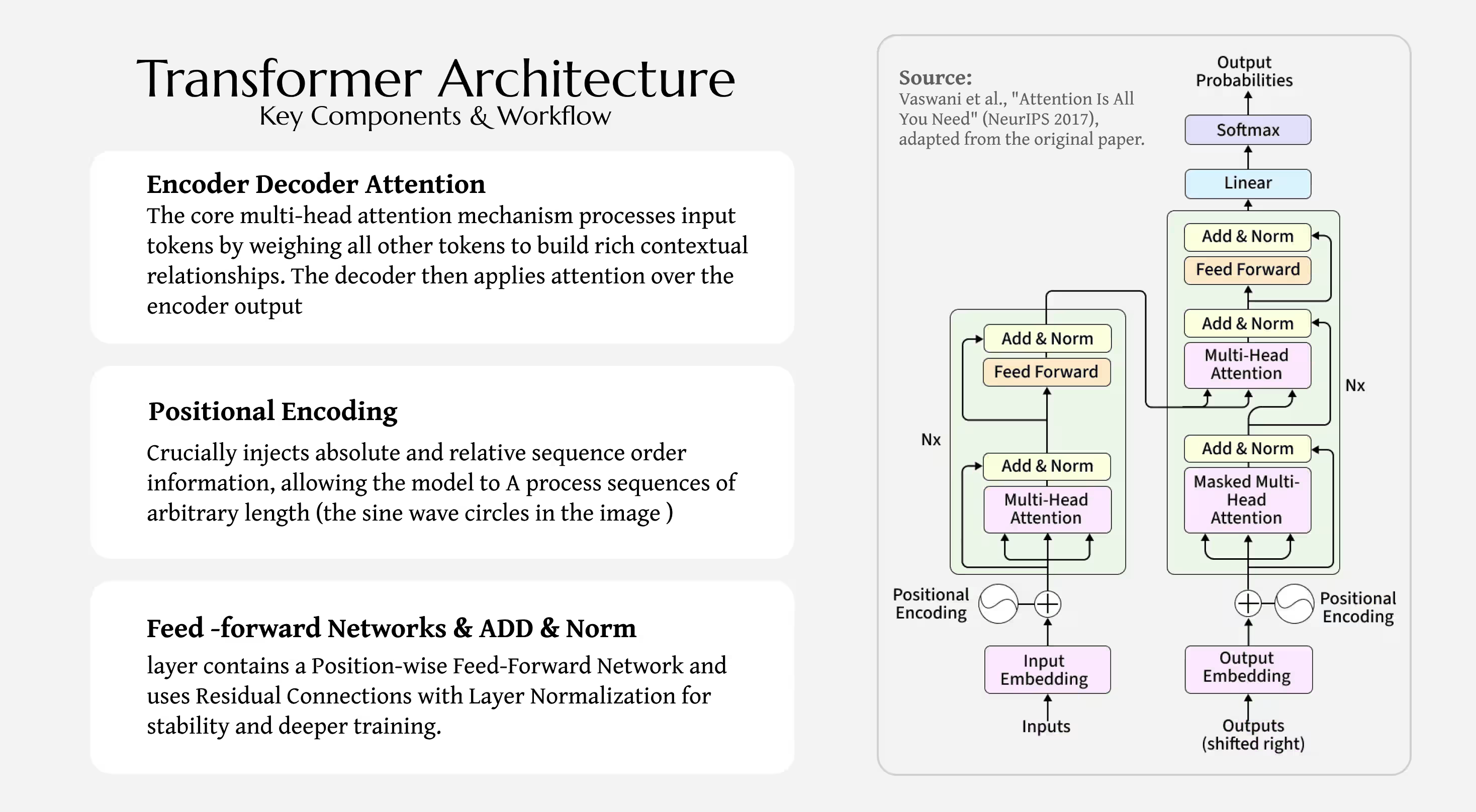
The original Transformer, described in "Attention Is All You Need," consists of two main components: an encoder and a decoder. They have the same architecture internally, but serve different purposes.
The encoder processes the input sequence and produces a contextualized representation of each token. Crucially, the encoder can attend to all tokens in the input at once-there are no restrictions on which tokens can attend to which.
The decoder processes the output sequence and generates predictions for the next token. But there's a constraint: a token at position \( i \) in the output should not attend to tokens at positions \( >i \). Why? Because during generation, those future tokens don't exist yet. This constraint is enforced using a "causal mask" (also called an autoregressive mask), which sets attention weights to zero for future positions.
Additionally, the decoder has cross-attention layers, where the decoder attends to the encoder's output. This allows the decoder to incorporate information from the input sequence when generating the output.
The original Transformer was designed for sequence-to-sequence tasks like machine translation. You feed in an English sentence to the encoder, and the decoder generates a French translation token by token, attending to the encoder output and previously generated tokens.
8.2 Decoder-Only Architectures
Many modern language models (GPT, Claude, Llama) use a decoder-only architecture. They dispense with the encoder and use only the decoder, with causal masking. This simplifies the architecture and is sufficient for a wide range of tasks.
The causal mask ensures that when predicting token \( i \), the model can only attend to tokens 1 through \( i-1 \). This maintains causality: the model doesn't cheat by looking at the token it's supposed to predict.
8.3 Complete Forward Pass
Let's trace a complete forward pass through a decoder-only Transformer:
- Embedding: Convert input token IDs to embeddings. If the vocabulary has 50,000 tokens, each embedding is a vector in \( \mathbb{R}^{512} \) (for a 512-dimensional model).
- Positional Encoding: Add positional encodings to account for token positions in the sequence.
- Transformer Layers (repeated): For each of \( L \) layers (e.g., \( L = 24 \)):
- Multi-Head Attention: Compute attention weights and produce context-aware token representations.
- Residual + LayerNorm: Add the input back and apply layer normalization.
- Feed-Forward: Apply the two-layer feed-forward network.
- Residual + LayerNorm: Add the residual and normalize again.
- Final Layer Norm: Apply one more layer normalization to the output of the final Transformer layer.
- Linear Projection to Logits: Project the final representations to vocabulary size (50,000). The result is logits-raw scores for each token.
- Softmax: Convert logits to probabilities. The output is a probability distribution over the vocabulary for each position.
During training, we compare these probabilities to the ground truth (the actual next tokens) using cross-entropy loss. During inference, we sample from the distribution (or take the argmax) to generate the next token, then append it to the input and repeat.
8.3b Full Transformer Decoder Block in PyTorch
import torch
import torch.nn as nn

class TransformerDecoderBlock(nn.Module):
    """Single decoder-only Transformer layer (GPT-style)."""

    def __init__(self, d_model: int = 512, n_heads: int = 8,
                 d_ff: int = 2048, dropout: float = 0.1):
        super().__init__()
        assert d_model % n_heads == 0

        # ── Multi-head self-attention ───────────
        self.attn   = nn.MultiheadAttention(d_model, n_heads,
                                            dropout=dropout,
                                            batch_first=True)
        # ── Feed-forward network ────────────────
        self.ff     = nn.Sequential(
            nn.Linear(d_model, d_ff),
            nn.GELU(),                  # smoother than ReLU
            nn.Dropout(dropout),
            nn.Linear(d_ff, d_model),
        )
        # ── Pre-norm (modern default, more stable than post-norm) ─
        self.norm1  = nn.LayerNorm(d_model)
        self.norm2  = nn.LayerNorm(d_model)
        self.drop   = nn.Dropout(dropout)

    def forward(self, x: torch.Tensor) -> torch.Tensor:
        """
        x: (batch, seq_len, d_model)
        Returns same shape.
        """
        T = x.size(1)
        # Causal mask: upper triangle → -inf so future tokens are invisible
        causal_mask = torch.triu(
            torch.ones(T, T, device=x.device, dtype=torch.bool), diagonal=1
        )

        # Pre-norm → attention → residual
        h = self.norm1(x)
        h, _ = self.attn(h, h, h, attn_mask=causal_mask)
        x = x + self.drop(h)

        # Pre-norm → feed-forward → residual
        x = x + self.drop(self.ff(self.norm2(x)))
        return x


# ── Minimal usage ───────
if __name__ == "__main__":
    block  = TransformerDecoderBlock(d_model=512, n_heads=8)
    tokens = torch.randn(2, 128, 512)   # batch=2, seq=128, dim=512
    out    = block(tokens)
    print(out.shape)                     # → torch.Size([2, 128, 512])
8.4 Parameter Count
How many parameters does a Transformer have? Let's count for a model with embedding dimension \( d \), vocabulary size \( V \), and \( L \) layers:
- Token embeddings: \( V \times d \)
- Per layer (× \( L \) layers):
- Multi-head attention: \( 3 d^2 + d^2 = 4 d^2 \) (for queries, keys, values, and output projection)
- Feed-forward: \( d \times 4d + 4d \times d = 8 d^2 \)
- Layer norm: \( 2d \) (per layer, negligible)
- Output layer: \( d \times V \)
The dominant term is the feed-forward networks: \( L \times 8 d^2 \). For GPT-3 with \( d = 12288 \) and \( L = 96 \), this alone is \( 96 \times 8 \times 12288^2 \approx 116 \) billion parameters. Adding token embeddings and other components brings the total to 175 billion parameters-one of the largest language models trained to date.
9. Training and Scaling
9.1 Next Token Prediction
Transformers are trained using unsupervised learning: predicting the next token given previous tokens. This is called the "next token prediction" or "language modeling" objective. The loss is:
\[ \mathcal{L} = -\frac{1}{N} \sum_{i=1}^{N} \log p_{\theta}(\text{token}_i | \text{token}_1, \ldots, \text{token}_{i-1}) \]where \( p_{\theta} \) is the model's predicted probability distribution (the output of the softmax layer) and \( N \) is the total number of tokens in the training data. The log probability ensures that the model is penalized more heavily for wrong predictions that were very confident.
This simple objective, when trained on massive amounts of data (hundreds of billions of tokens), leads to models that can perform a remarkably wide range of tasks: translation, question answering, code generation, reasoning, and much more. This is one of the most surprising findings in modern AI: training for next token prediction is sufficient to learn a powerful general-purpose model.
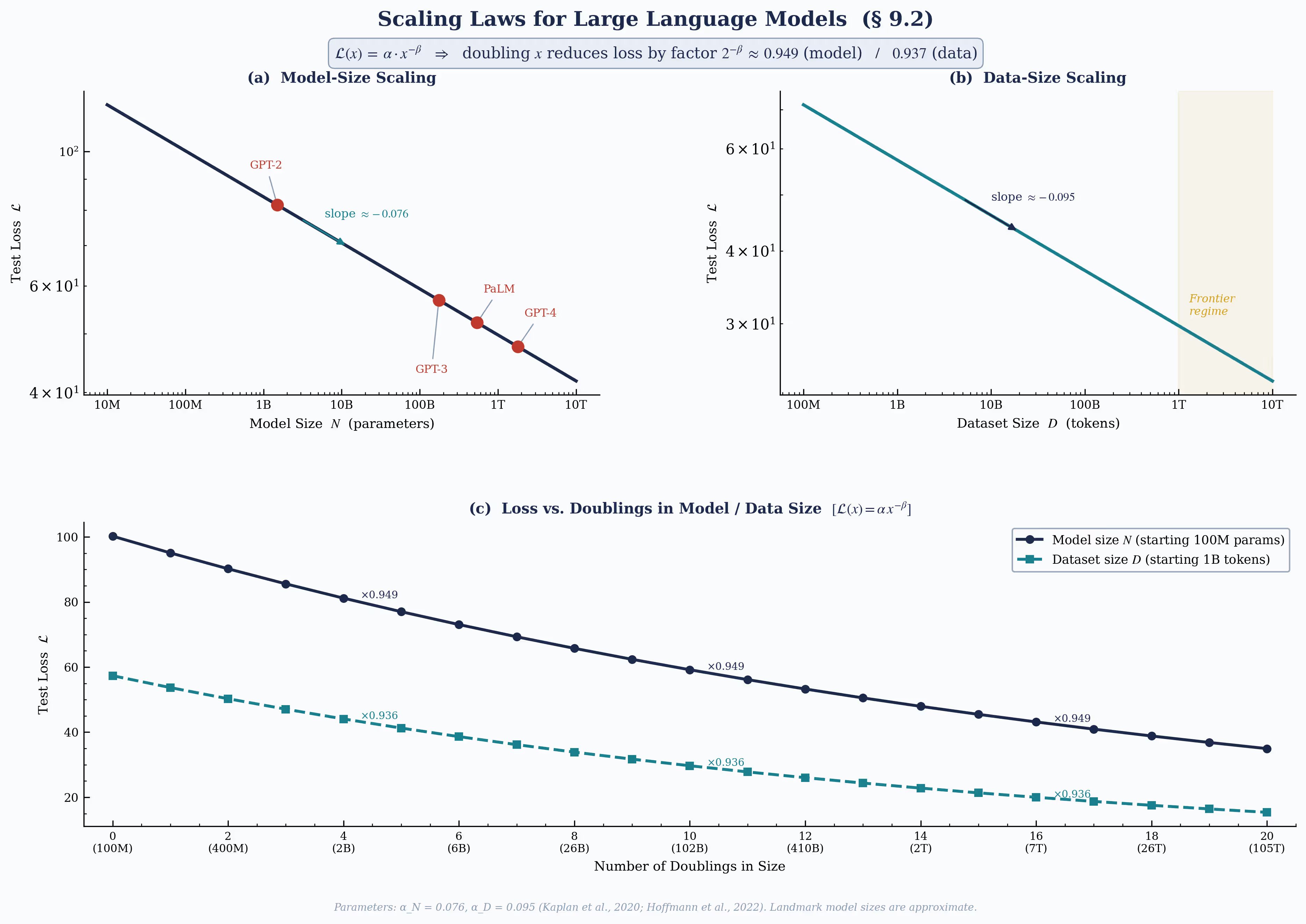
9.2 Scaling Laws
A key empirical finding is that larger models trained on more data perform better, following a smooth power law. In other words, if you double the model size (double the number of parameters and training tokens), the loss decreases approximately by a constant factor. This allows researchers to predict the performance of larger models based on smaller experiments.
The scaling law is often written as:
\[ \mathcal{L}(N) = a N^{-b} \]where \( N \) is some measure of model or data size, and \( a \) and \( b \) are constants. Empirically, \( b \approx 0.07 \) for doubling model size and similar values for data scaling. This suggests that, at least in the regime we've explored so far, there's no fundamental limit to how good these models can be-we just need to scale up.
This finding has profound implications. It suggests that engineering better data, training longer, and building larger models are the primary levers for improving AI. In contrast to some earlier beliefs that we'd hit a fundamental ceiling, scaling laws suggest that improvements might continue for years.
9.3 Training Efficiency and Hardware
Training large Transformers requires specialized hardware. GPUs (like NVIDIA's A100) and custom hardware (like Google's TPUs) are essential because they can perform the large matrix multiplications that dominate Transformer computation in parallel. A single GPU can be used for a model, but for large models, multiple GPUs are coordinated to train the model in parallel.
Data parallelism and model parallelism are the two main approaches. With data parallelism, each GPU processes a different batch of data and computes gradients independently, which are then averaged. With model parallelism, different parts of the model live on different GPUs, and data passes through them in sequence. For the largest models, a combination of both is used.
Efficient training also requires careful use of lower precision arithmetic. Most modern models are trained in mixed precision: using 16-bit floating-point (half precision) for the forward and backward passes, and 32-bit floating-point (full precision) for maintaining the model parameters and optimizer states. This reduces memory usage and computation time without significantly affecting model quality.
9.4 Inference and Context Windows
After training, we use the model for inference: generating text given a prompt. One limitation of the standard Transformer is the quadratic cost of attention with respect to sequence length. For a context window of 2048 tokens, the attention computation is manageable. But for context windows of 100,000 tokens (as in some recent models), the \( O(n^2) \) cost becomes prohibitive.
Several techniques have been proposed to extend context windows:
- Sparse attention: Instead of computing attention between all pairs of tokens, compute it only for a subset (e.g., local attention within a window, or strided attention). This reduces cost to \( O(n \log n) \) or \( O(n) \).
- Approximate attention: Use low-rank approximations or kernel tricks to approximate the full attention matrix more cheaply.
- Retrieval augmentation: Instead of increasing the context window, retrieve the most relevant documents and feed them with the query. This is more efficient than processing a huge context.
- Sliding window attention: Combine local attention (attending to nearby tokens) with occasional long-range attention to distant tokens, balancing cost and expressiveness.
The tradeoff between context length and computational cost remains an active area of research.
10. Beyond the Original Transformer
10.1 Decoder-Only Models
The original Transformer was an encoder-decoder architecture. But modern large language models-GPT, Claude, Llama-use a decoder-only architecture. The decoder is more efficient for left-to-right generation (the standard way language models work), and removing the encoder simplifies training and inference.
10.2 Attention Variants
As models have scaled, limitations of standard attention have become apparent. For very long sequences (100k+ tokens), the quadratic cost becomes prohibitive. Research has explored:
- Multi-Query Attention: Use a single set of key-value pairs shared across all query heads, reducing memory and computation.
- Grouped Query Attention: A compromise between multi-head (multiple key-value pairs per head) and multi-query (single pair), improving speed while maintaining quality.
- Flash Attention: A careful algorithmic redesign that reorders computations to maximize cache hits, achieving 2-4x speedups on modern GPUs.
10.3 Learned vs. Fixed Positional Encodings
While the original Transformer uses sinusoidal positional encodings, many modern models (including BERT and others) use learned positional embeddings. These are simpler and can be fine-tuned by the model. The tradeoff: learned encodings don't generalize to longer sequences than seen during training, while sinusoidal encodings do.
10.4 Alternative Activation Functions
The original Transformer uses ReLU in the feed-forward layer. Many recent models use GELU (Gaussian Error Linear Unit):
\[ \text{GELU}(x) = x \Phi(x) \]where \( \Phi \) is the cumulative distribution function of the standard normal distribution. GELU is smoother than ReLU and has been found to improve performance. Other alternatives include SwiGLU and variants.
10.5 Normalization Variants
Pre-normalization (applying layer norm before rather than after the layer) has become standard in recent models, improving training stability. Root Mean Square Layer Normalization (RMSNorm) is a simpler variant that has been adopted in some recent large models.
10.6 Architectural Innovations: Vision Transformers, Sparse Transformers, Conditional Computation
The Transformer architecture has been adapted for numerous domains beyond language:
- Vision Transformers (ViT): Apply the Transformer architecture to images by dividing them into patches and treating patches as tokens. This has become competitive with convolutional neural networks for image classification.
- Sparse Transformers: Use sparse attention patterns (e.g., attending to local windows and logarithmic-distance positions) to reduce the quadratic cost.
- Conditional Computation: Some tokens or layers are only computed when necessary, similar to mixture-of-experts models, reducing total computation.
These variants show that the core ideas of attention and Transformer architecture are general and can be adapted to different domains and constraints.
11. Conclusion
The Transformer is a remarkable architecture. It solved the central problem of neural sequence modeling-how to relate distant tokens efficiently-through the elegant mechanism of self-attention. By stacking attention layers with residual connections and feed-forward networks, the Transformer can learn from billions of tokens and capture complex patterns in language, vision, and other domains.
But the Transformer is not a finished product. Despite its success, we still don't fully understand why it works so well, why scaling laws hold, or what the fundamental limits of the architecture are. Researchers continue to propose variants: sparser attention, alternative normalization schemes, and architectural innovations.
What we do know is this: the Transformer, combined with next-token prediction and scale, has proven to be a remarkably effective recipe for building general-purpose AI systems. It is the foundation of modern language models, and understanding it deeply is essential for anyone working in machine learning or AI.
The journey from the sequence problem to self-attention to the full Transformer architecture is a journey of constant refinement and elegance. Each component-attention, positional encoding, layer normalization, residual connections-serves a purpose that we've explored in detail. By understanding these components individually and how they fit together, you now have the foundation to read research papers, implement Transformers yourself, and contribute to the next generation of AI systems.
Transformer Components at a Glance
| Component | Purpose | Complexity | Learnable Parameters |
|---|---|---|---|
| Token Embedding | Convert token IDs to dense vectors | O(1) | \(V \times d\) |
| Positional Encoding | Encode sequence position information | O(1) sinusoidal or O(\(n \times d\)) learned | 0 (sinusoidal) or \(n \times d\) (learned) |
| Multi-Head Attention | Relate tokens across sequence | O(\(n^2 d\)) | \(4d^2\) (Q, K, V, O projections) |
| Feed-Forward Network | Per-token nonlinear transformation | O(\(n d^2\)) | \(8d^2\) (two linear layers + biases) |
| Layer Normalization | Stabilize and normalize activations | O(\(nd\)) | \(2d\) (scale and shift) |
| Residual Connection | Enable gradient flow in deep networks | O(1) | 0 (no learnable parameters) |
Frequently Asked Questions
- Absolutely. This article teaches the mathematics as it becomes necessary, beginning with intuition and building to formal derivations. A background in calculus and linear algebra is helpful but not required-the article explains everything from first principles.
- Self-attention allows tokens to attend to all other tokens in the same sequence. Cross-attention (used in encoder-decoder Transformers) allows the decoder to attend to the encoder's output. For decoder-only models like GPT, only self-attention with causal masking is used.
- Dot products in high-dimensional spaces can produce very large values. Scaling by √d (the embedding dimension) keeps the variance of dot products stable around 1, preventing the softmax from becoming too peaked or too flat, which improves gradient flow during training.
- Approximately 45-60 minutes if read continuously. We recommend reading one major section per session and working through the examples. Taking time to understand each concept deeply is more valuable than rushing through.
- Yes. The article includes worked examples, mathematical derivations, and explanations of every component. By the end, you will understand each operation sufficiently to implement a working Transformer using PyTorch or NumPy.
- RNNs process sequences sequentially, compressing information through hidden states that can degrade over distance. Transformers use self-attention, which allows each token to directly compare with any other token regardless of distance, with no intermediate compression.
- Causal masking prevents tokens from attending to future tokens in the sequence. During training and generation, we only have access to past tokens, so causal masking ensures the model only uses available information, maintaining the autoregressive (left-to-right) generation property.
- Yes. Transformers remain the foundation of state-of-the-art language models, multimodal models, and vision models. While variants and extensions have been proposed (like sparse attention, mixture-of-experts), the core Transformer architecture remains central to modern AI.