
Uniform Distribution
Abstract
A complete, visual guide to the Uniform distribution: what it is, the flat-density formula behind it, notation and parameters, the discrete and continuous forms, symmetry and other core properties, moments and the moment generating function, the cumulative distribution function, a worked example, order statistics, sums of uniform variables, related distributions, how uniform random numbers are generated on a computer, and where the distribution shows up in statistics, simulation and machine learning.
What Is a Uniform Distribution?
In probability theory and statistics, the uniform distribution (also called the rectangular distribution) is a probability distribution in which every outcome within a defined range is equally likely. Unlike distributions such as the normal distribution, whose density piles up around a central value, the uniform distribution has a perfectly flat density (or, in the discrete case, equal probability mass) across its entire support, and zero probability outside it. It comes in two forms: the continuous uniform distribution, defined over an interval of real numbers, and the discrete uniform distribution, defined over a finite set of distinct outcomes (see Discrete Uniform Distribution below).
A random variable \( X \) that follows a continuous uniform distribution on the interval \( [a,b] \) is said to be uniformly distributed. The distribution is the simplest possible model of "complete ignorance within known bounds": if all that is known about a quantity is its minimum and maximum, and there is no reason to favor any value over another, the uniform distribution is the least-assuming choice (formalized later under maximum entropy). It is also, in practice, the distribution computers generate natively—nearly every other kind of randomness used in simulation and machine learning is built by transforming uniform draws (see Generating Uniform Random Numbers).
The Formula
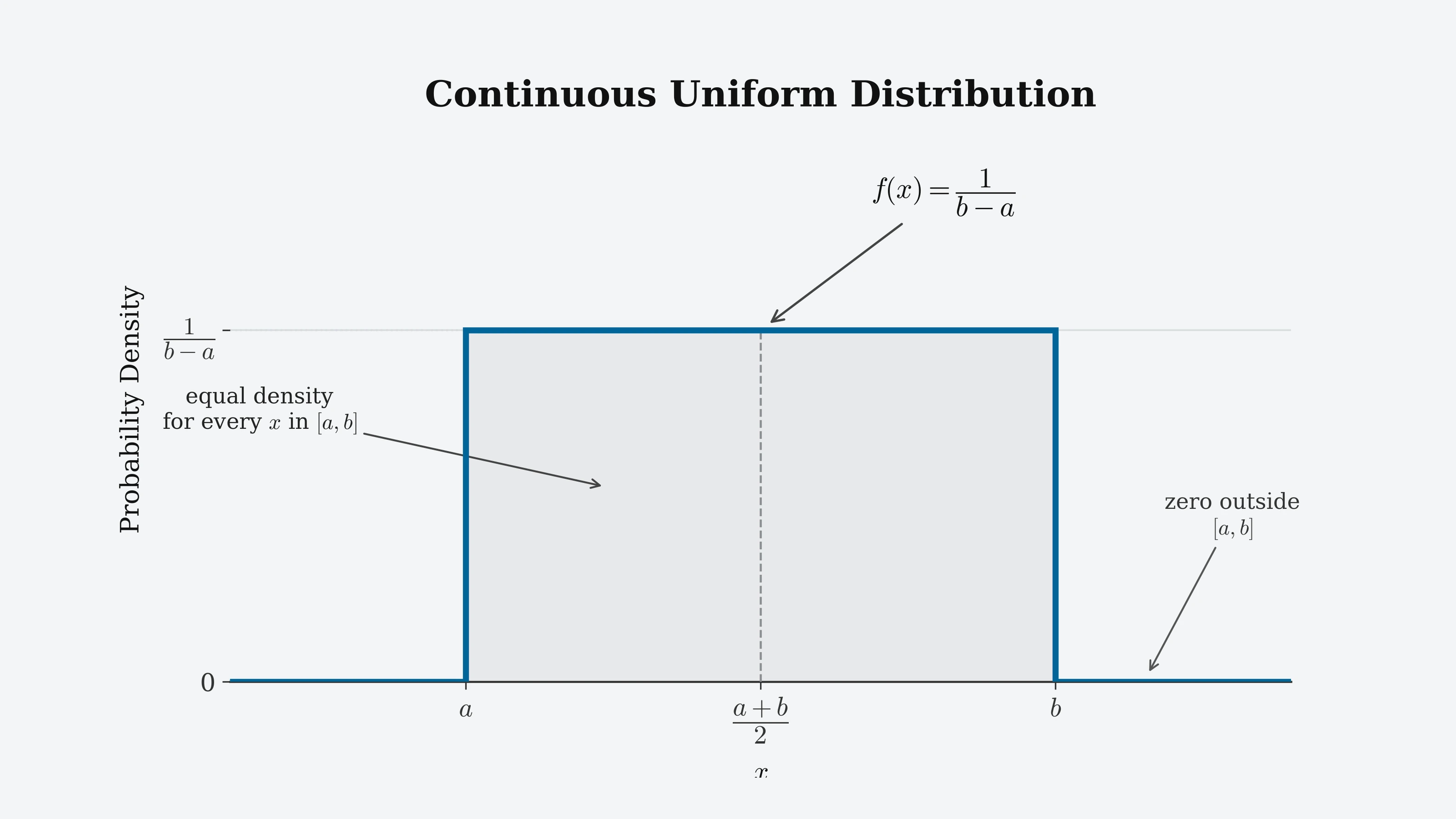
The probability density function (PDF) of a continuous uniform distribution on the interval \( [a, b] \) is:
\[ f(x) = \begin{cases} \dfrac{1}{b-a} & \text{for } a \le x \le b \\[6pt] 0 & \text{otherwise} \end{cases} \]Here \( a \) is the lower bound of the support, \( b \) is the upper bound, and \( b - a \) is the width of the interval. The density is a constant, \( 1/(b-a) \), everywhere inside \( [a,b] \), and exactly zero everywhere outside it—there is no tapering, no tails, and no single most likely value. The total area under the curve is the width of the interval multiplied by its constant height, \( (b-a) \times \frac{1}{b-a} = 1 \), confirming the density integrates to \( 1 \) as required of any valid PDF.
The two parameters \( a \) and \( b \) are all that is needed to fully specify the distribution. Whether the endpoints \( a \) and \( b \) are themselves included in the support is a minor technicality for the continuous case: because any single point has probability zero under a continuous density, it makes no difference to any probability calculation whether the interval is written as closed \( [a,b] \), open \( (a,b) \), or half-open.
Notation & Parameters
A continuous uniform distribution with lower bound \( a \) and upper bound \( b \) is written compactly as:
\[ X \sim U(a, b) \quad \text{or equivalently} \quad X \sim \mathcal{U}(a, b) \]read as "\( X \) is uniformly distributed between \( a \) and \( b \)." Several conventions and constraints apply:
- \( a, b \in \mathbb{R} \) can be any real numbers, provided \( a < b \). If \( a = b \) the distribution degenerates to a single point with no spread, which is not a valid continuous uniform distribution.
- The support of the distribution—the set of values \( X \) can take—is the bounded interval \( [a, b] \), unlike the normal distribution's unbounded support across all of \( \mathbb{R} \). Values outside \( [a,b] \) are not merely unlikely; they are strictly impossible.
- The special case \( U(0,1) \), the standard uniform distribution, is the default output of essentially every pseudo-random number generator and the starting point for generating other kinds of random variables (see Generating Uniform Random Numbers).
- Some sources instead parameterize by the midpoint \( m = (a+b)/2 \) and half-width \( h = (b-a)/2 \), writing the support as \( [m-h,\, m+h] \); this is equivalent but less common than the endpoint parameterization used throughout this article.
Discrete Uniform Distribution
The discrete uniform distribution is the finite-outcome counterpart to the continuous case: a random variable \( X \) that takes one of \( n \) distinct, equally likely values \( \{x_1, x_2, \ldots, x_n\} \) has probability mass function:
\[ P(X = x_i) = \frac{1}{n}, \qquad i = 1, 2, \ldots, n \]The canonical example is a fair six-sided die, where \( n = 6 \) and each face \( \{1,2,3,4,5,6\} \) occurs with probability \( 1/6 \). When the outcomes are the consecutive integers from \( a \) to \( b \) inclusive (so \( n = b - a + 1 \)), the distribution has closed-form mean and variance:
\[ E[X] = \frac{a+b}{2}, \qquad \operatorname{Var}(X) = \frac{(b-a+1)^2 - 1}{12} = \frac{n^2-1}{12} \]These mirror the continuous formulas closely (see Core Properties), with the variance differing only by the discreteness correction that shrinks as \( n \) grows. Other everyday examples of discrete uniform variables include a coin flip (\( n=2 \)), a shuffled card's rank (\( n=13 \)), and a lottery number drawn from a fixed range. Unless otherwise noted, the remainder of this article focuses on the continuous case, since it is the one with the richer mathematical structure and the wider role in statistics and simulation.
Core Properties
Beyond the formula and its two parameters, the uniform distribution has a set of defining mathematical properties that follow directly from its flat, bounded density.
Symmetry
The density \( f(x) \) is symmetric about the midpoint \( m = (a+b)/2 \): reflecting any point across the midpoint leaves the density unchanged, since the density is constant everywhere on the support in the first place. As with any symmetric distribution, this forces the skewness to zero (see below).
Mean, Median, and Midpoint Coincide
Because the density is flat and symmetric, the mean and median both land on the exact midpoint of the interval:
\[ E[X] = \frac{a+b}{2} \]Unlike the normal distribution, the uniform distribution has no single mode—every point in \( [a,b] \) is equally likely, so every point is, in a sense, tied for most probable. This absence of a peak is one of the clearest visual signatures distinguishing a uniform distribution from a bell-shaped one.
Variance and Standard Deviation
The variance depends only on the width of the interval, not on its location:
\[ \operatorname{Var}(X) = \frac{(b-a)^2}{12}, \qquad \sigma = \frac{b-a}{\sqrt{12}} = \frac{b-a}{2\sqrt{3}} \]Doubling the width of the interval quadruples the variance, since variance scales with the square of the spread. Shifting \( a \) and \( b \) by the same amount (translating the interval left or right) leaves the variance completely unchanged, just as with the normal distribution's mean parameter.
Skewness
Skewness measures the asymmetry of a distribution. Because the uniform distribution is perfectly symmetric about its midpoint, its skewness is exactly:
\[ \text{Skewness} = 0 \]This places it alongside the normal distribution as symmetric, even though the two shapes look nothing alike—a reminder that skewness alone does not distinguish flat distributions from peaked ones (see kurtosis below for the measure that does).
Kurtosis
Kurtosis describes how heavy or light a distribution's tails are relative to its peak. The uniform distribution has no tails at all—probability simply stops at \( a \) and \( b \)—and correspondingly has a kurtosis of:
\[ \text{Kurtosis} = \frac{9}{5} = 1.8, \qquad \text{Excess kurtosis} = 1.8 - 3 = -1.2 \]A negative excess kurtosis makes the uniform distribution platykurtic: flatter and lighter-tailed than the normal distribution, which serves as the excess-kurtosis baseline of zero. Among common distributions, the uniform distribution's excess kurtosis of \( -1.2 \) is close to the most negative value achievable by any distribution, reflecting how little probability mass it places anywhere outside a hard, finite boundary.
No Single Mode; Constant Density
Where the normal distribution has one clear peak and two inflection points, the uniform distribution's density has neither: \( f(x) \) is constant on the interior of \( [a,b] \), so its derivative is zero everywhere it is defined, and the only "features" of the curve are the two discontinuous jumps at \( x=a \) and \( x=b \), where the density steps instantly from \( 0 \) up to \( 1/(b-a) \) and back down to \( 0 \).
Maximum Entropy
Among all continuous probability distributions supported on a fixed, finite interval \( [a,b] \) and nothing else, the uniform distribution is the one with maximum entropy: it is the distribution that assumes the least additional structure beyond the bounds themselves, spreading probability as evenly as those bounds allow. This is the formal justification for treating a bounded quantity as uniform when only its minimum and maximum are known—the same role the normal distribution plays when only the mean and variance are known.
Closure Under Linear Transformations
Uniform distributions behave predictably under scaling and shifting:
\[ X \sim U(a,b) \implies cX + d \sim U(ca+d,\, cb+d) \quad \text{for } c > 0 \]The family of uniform distributions is closed under positive linear transformations: any interval can be stretched or shifted into any other interval and the result is still uniform on the new interval. This is why the standard uniform distribution \( U(0,1) \) is sufficient to generate a uniform distribution over any other interval by a simple rescaling, \( X = a + (b-a)U \) (see Generating Uniform Random Numbers). Unlike the normal distribution, however, summing two independent uniform variables does not produce another uniform distribution—see Sums of Uniform Variables below.
Moments & Generating Functions
Beyond the mean and variance, distributions are characterized by their full sequence of moments. For the standard uniform distribution \( U(0,1) \), the raw moments about the origin follow an especially simple pattern:
| Order \( p \) | Raw moment \( E[X^p] \) |
|---|---|
| 0 | \( 1 \) |
| 1 | \( 1/2 \) (the mean) |
| 2 | \( 1/3 \) |
| 3 | \( 1/4 \) |
| 4 | \( 1/5 \) |
| 5 | \( 1/6 \) |
| 6 | \( 1/7 \) |
This pattern, \( E[X^p] = 1/(p+1) \), falls directly out of integrating the constant density \( x^p \cdot 1 \, dx \) over \( [0,1] \). For the general interval \( [a,b] \), the central moments (about the mean) also take a clean closed form: all odd-order central moments vanish, a consequence of symmetry, while the even-order moments are:
\[ E\!\left[(X - \mu)^{2k}\right] = \frac{(b-a)^{2k}}{2^{2k}(2k+1)} \]The moment generating function (MGF) encodes every moment of a distribution at once. For a uniform distribution on \( [a,b] \), it is:
\[ M(t) = E\left[e^{tX}\right] = \frac{e^{tb} - e^{ta}}{t(b-a)}, \qquad M(0) = 1 \]The expression is undefined at \( t=0 \) in this raw form (division by zero), but its limit as \( t \to 0 \) correctly equals \( 1 \), consistent with the general fact that \( M(0) = 1 \) for any distribution. Unlike the normal distribution's MGF, which is a clean exponential of a quadratic, the uniform distribution's MGF has no such simplification—a reflection of the fact that a flat density is, in a precise sense, a much less "natural" object for the exponential/Fourier machinery underlying moment generating functions than the bell curve is.
Finally, the differential entropy of a uniform distribution on \( [a,b] \)—the quantity maximized subject to a fixed support, as noted above—has the closed form:
\[ H(X) = \ln(b-a) \]The entropy depends only on the width \( b-a \), not on the interval's location, and grows without bound as the interval widens—a wider range of equally likely outcomes is, intuitively, less predictable and therefore carries more entropy.
Cumulative Distribution Function
The PDF \( f(x) \) (see the formula above) gives the constant density of values near \( x \) but does not itself give a probability. The probability that \( X \) falls at or below some threshold is given instead by the cumulative distribution function (CDF), written \( F(x) \): the area under the flat PDF up to \( x \).
Because the density is constant, the CDF of a uniform distribution on \( [a,b] \) is piecewise linear—a straight ramp rising from \( 0 \) to \( 1 \):
\[ F(x) = \begin{cases} 0 & x < a \\[4pt] \dfrac{x-a}{b-a} & a \le x \le b \\[6pt] 1 & x > b \end{cases} \]This is a marked contrast to the normal distribution's S-shaped CDF (see the normal distribution's CDF), which has no closed form and requires the error function to evaluate. The uniform CDF, by contrast, is one of the simplest closed-form CDFs in all of probability theory—a direct consequence of integrating a constant.
- \( F(a) = 0 \), since no probability mass lies below the lower bound,
- \( F\!\left(\frac{a+b}{2}\right) = 0.5 \) exactly, since the interval's midpoint splits the probability mass evenly (a consequence of symmetry), and
- \( F(b) = 1 \), since all probability mass lies at or below the upper bound.
To find the probability that a uniform variable \( X \) falls strictly between two values \( c \) and \( d \) within \( [a,b] \), subtract the two CDF values—which, thanks to the linear form, reduces to a simple ratio of lengths:
\[ P(c < X \le d) = F(d) - F(c) = \frac{d-c}{b-a} \]This "probability equals proportion of length" rule is the defining intuition of the uniform distribution: the chance of landing in any sub-interval depends only on that sub-interval's width, never on its position within \( [a,b] \).
Worked Example
Suppose a bus is scheduled to arrive at a stop, and its actual arrival time (in minutes after the scheduled time) is uniformly distributed between \( a = 0 \) and \( b = 20 \) minutes. What is the probability the bus arrives more than 15 minutes late?
Step 1 — Identify the interval: here \( X \sim U(0, 20) \), so the density is constant at \( 1/(20-0) = 1/20 \) across the whole range.
Step 2 — Apply the length-ratio rule: the event "more than 15 minutes late" corresponds to the sub-interval \( (15, 20] \), which has length \( 20 - 15 = 5 \).
\[ P(X > 15) = \frac{20 - 15}{20 - 0} = \frac{5}{20} = 0.25 \]There is a 25% chance the bus arrives more than 15 minutes late. Unlike the normal distribution's worked example, no standardization or table lookup is required—every uniform-distribution probability reduces to this same length-ratio calculation.
Second question: within what interval, centered on the mean, do the middle 50% of arrival times fall? Since the distribution is symmetric, the middle 50% is centered on the mean \( (a+b)/2 = 10 \) and spans 50% of the total width on each side of that center, i.e. the middle half of the full interval:
\[ \left[10 - \tfrac{1}{4}(20),\ \ 10 + \tfrac{1}{4}(20)\right] = [5,\ 15] \]The middle 50% of arrival times falls between 5 and 15 minutes late.
Order Statistics
If \( n \) independent draws \( X_1, \ldots, X_n \) are taken from a standard uniform distribution \( U(0,1) \) and then sorted from smallest to largest, \( X_{(1)} \le X_{(2)} \le \cdots \le X_{(n)} \), the resulting sorted values are called the order statistics of the sample. Remarkably, the \( k \)-th order statistic follows an exact Beta distribution:
\[ X_{(k)} \sim \operatorname{Beta}(k,\, n-k+1) \]with mean \( E[X_{(k)}] = k/(n+1) \). Intuitively, the \( n \) points divide the unit interval into \( n+1 \) gaps, and by symmetry each gap has expected length \( 1/(n+1) \), so the \( k \)-th smallest point sits at an expected distance of \( k/(n+1) \) from the origin. This result underlies methods such as plotting positions in probability plots and the construction of non-parametric confidence bands, and is the reason the uniform distribution is described in the next section as a special case of the Beta family.
Sums of Uniform Variables
Unlike the normal distribution, which is closed under addition (see the normal distribution's closure property), summing two or more independent uniform variables does not produce another uniform distribution. The sum of \( n \) independent \( U(0,1) \) variables follows the Irwin–Hall distribution, a piecewise-polynomial distribution supported on \( [0, n] \) with density:
\[ f_n(x) = \frac{1}{(n-1)!}\sum_{k=0}^{\lfloor x \rfloor} (-1)^k \binom{n}{k} (x-k)^{n-1} \]For \( n=2 \), this reduces to a simple triangular density peaking at \( x=1 \) — the well-known fact that summing two dice or two uniform draws produces a distribution that clusters near the middle of its range and tapers toward the extremes, rather than staying flat. As \( n \) grows, the shape of the Irwin–Hall density rapidly approaches a normal bell curve, a direct and easily visualized illustration of the central limit theorem: even though each individual uniform draw is perfectly flat, sums of many such draws are approximately Gaussian. In fact, summing just twelve independent \( U(0,1) \) variables and subtracting 6 was, for decades, a standard trick for generating approximately normal random numbers on early computers, before more accurate methods such as Box–Muller became standard (see Generating Normal Random Numbers).
Generating Uniform Random Numbers
Unlike most named distributions, the uniform distribution is not itself typically generated by transforming something else—it is the starting point. Computers produce uniform randomness directly via pseudo-random number generators (PRNGs), deterministic algorithms that produce long sequences of numbers which pass statistical tests for uniformity and independence, seeded from an initial value:
- Linear congruential generators — among the oldest and simplest PRNGs, producing each output from the previous one via \( x_{n+1} = (c \cdot x_n + d) \bmod m \). Fast but with known statistical weaknesses, so they are largely obsolete for serious simulation work today.
- Mersenne Twister — a widely used generator with an extremely long period and good statistical properties, historically the default in many programming languages and numerical libraries, though newer algorithms have since surpassed it in some benchmarks.
- Cryptographically secure PRNGs (CSPRNGs) — generators such as those built on ChaCha20 or AES, designed so that observing part of the output sequence gives no practical advantage in predicting future values; required for security-sensitive applications such as key generation, unlike general-purpose simulation PRNGs.
Once a stream of standard uniform values \( U(0,1) \) is available, it becomes the raw material for generating almost any other distribution, most directly through inverse transform sampling: given a target distribution's CDF \( F \), drawing \( u \sim U(0,1) \) and computing \( x = F^{-1}(u) \) produces a random variate from that target distribution. This is exactly how the normal distribution's random-number generators and the exponential-distribution transform mentioned above are constructed. Libraries such as NumPy (numpy.random.uniform()) or PyTorch (torch.rand()) expose this base uniform generator directly, on top of which every other random-sampling function in those libraries is ultimately built.
A Short History
Unlike the normal distribution, whose discovery is credited to specific 18th- and 19th-century mathematicians (see the normal distribution's history), the uniform distribution has no comparable single point of discovery—its idea is older than probability theory's formal development and arguably implicit in the very earliest treatments of games of chance, where dice, coins, and cards are naturally modeled as equally-likely outcomes.
Early probabilists such as Gerolamo Cardano in the 16th century and later Fermat and Pascal in their famous 1654 correspondence on the "problem of points" all implicitly relied on discrete uniform assumptions—that each face of a die or each possible card is equally likely—without needing to name or formalize the concept as a distribution.
The formal, axiomatic articulation of a continuous uniform distribution had to wait for the broader development of measure-theoretic probability in the early 20th century, principally through Andrey Kolmogorov's 1933 axiomatization of probability theory, which provided the rigorous foundation needed to define probability densities—including constant ones—on general continuous spaces.
The distribution's modern importance owes less to any single theoretical result and more to the rise of digital computing in the mid-20th century: once machines needed a source of "randomness" for Monte Carlo simulation, and computer scientists such as John von Neumann and later D. H. Lehmer (who introduced the linear congruential generator in 1949) began engineering algorithms to approximate it, the uniform distribution became the practical bedrock on which essentially all computational randomness is built (see Generating Uniform Random Numbers).
Where It Shows Up
The uniform distribution's occurrence in practical problems falls loosely into a few categories: cases where physical or procedural symmetry genuinely makes every outcome equally likely, cases where it is used as a deliberate maximum-entropy default under bounded ignorance, and its foundational role as the raw source of computational randomness. A selection of concrete examples across each category:
- Random number generation — the base output of virtually every PRNG, from which other distributions are derived via inverse transform sampling (see Generating Uniform Random Numbers).
- Monte Carlo simulation — numerical integration and probabilistic simulations typically begin from uniform draws before transforming them into whatever distribution the model requires.
- Cryptography — secure key generation, nonces, and salts rely on values drawn (via CSPRNGs) as close to uniformly at random as possible, since predictability directly undermines security.
- Games of chance — dice, roulette wheels, shuffled decks, and lottery draws are all designed and modeled as discrete uniform distributions over their possible outcomes.
- Rounding error — the error introduced by rounding a continuous measurement to the nearest unit is conventionally modeled as uniform on \( [-0.5, 0.5] \) of that unit.
- Bayesian priors — a uniform distribution over a parameter's plausible range is a standard "uninformative" or "flat" prior when no outcome should be favored in advance, directly invoking the maximum-entropy property discussed above.
- Scheduling and queuing models — arrival times within a fixed window (such as the bus example in the worked example above) are commonly approximated as uniform when no part of the window is more likely than another.
- Machine learning initialization — neural network weights are frequently initialized by drawing from a uniform distribution over a small symmetric interval, such as in Xavier/Glorot initialization, before training adjusts them.
Uniform distributions are sometimes misapplied to data that only looks evenly spread over a limited sample but is not, in fact, flat over its true range. When a variable is known to cluster around a typical value, or when its range is not sharply bounded, a distribution built for that purpose — such as the normal, triangular, or Beta distribution — is generally more appropriate than forcing a uniform assumption for the sake of simplicity.
Frequently Asked Questions
- It is a probability distribution in which every outcome, or every value in an interval, is equally likely; the probability density (or probability mass) is perfectly flat across the entire range.
- A discrete uniform distribution assigns equal probability to a finite set of distinct outcomes, such as the faces of a die. A continuous uniform distribution assigns equal probability density to every real number within an interval [a, b], such as a random number generated between 0 and 1.
- For a continuous uniform distribution on [a, b], the mean is (a + b) / 2, the exact midpoint of the interval, and the variance is (b - a)^2 / 12.
- Pseudo-random number generators natively produce values from a uniform distribution on (0, 1); nearly every other random variable used in simulation, cryptography, and machine learning is produced by transforming uniform draws, most directly via inverse transform sampling.
- Yes. Among all continuous distributions supported on a fixed, finite interval [a, b], the uniform distribution has the maximum entropy, making it the natural default when only the bounds of a variable are known and nothing else.
- A uniform distribution has a skewness of 0, since it is perfectly symmetric about its midpoint, and an excess kurtosis of -1.2, making it platykurtic (lighter-tailed and flatter than a normal distribution).
- Given a uniform random draw u on (0, 1) and the inverse CDF of any target distribution, computing that inverse CDF at u produces a random variate from the target distribution, which is the standard method for turning uniform randomness into any other kind.
- The uniform distribution is a special case of the Beta distribution with both shape parameters equal to 1, its order statistics follow Beta distributions, sums of independent uniforms approach normality via the Irwin-Hall distribution, and the discrete uniform distribution is the finite-outcome analogue used for dice, cards, and lottery draws.