
Normal (Gaussian) Distribution
Abstract
A complete, visual guide to the Normal (Gaussian) distribution: what it is, the formula behind the bell curve, notation and parameters, symmetry, skewness and kurtosis, the cumulative distribution function, the 68-95-99.7 empirical rule, the standard normal (z) table, a worked example, the central limit theorem, how parameters are estimated from data, related distributions, and where it shows up in statistics and machine learning.
What Is a Normal Distribution?
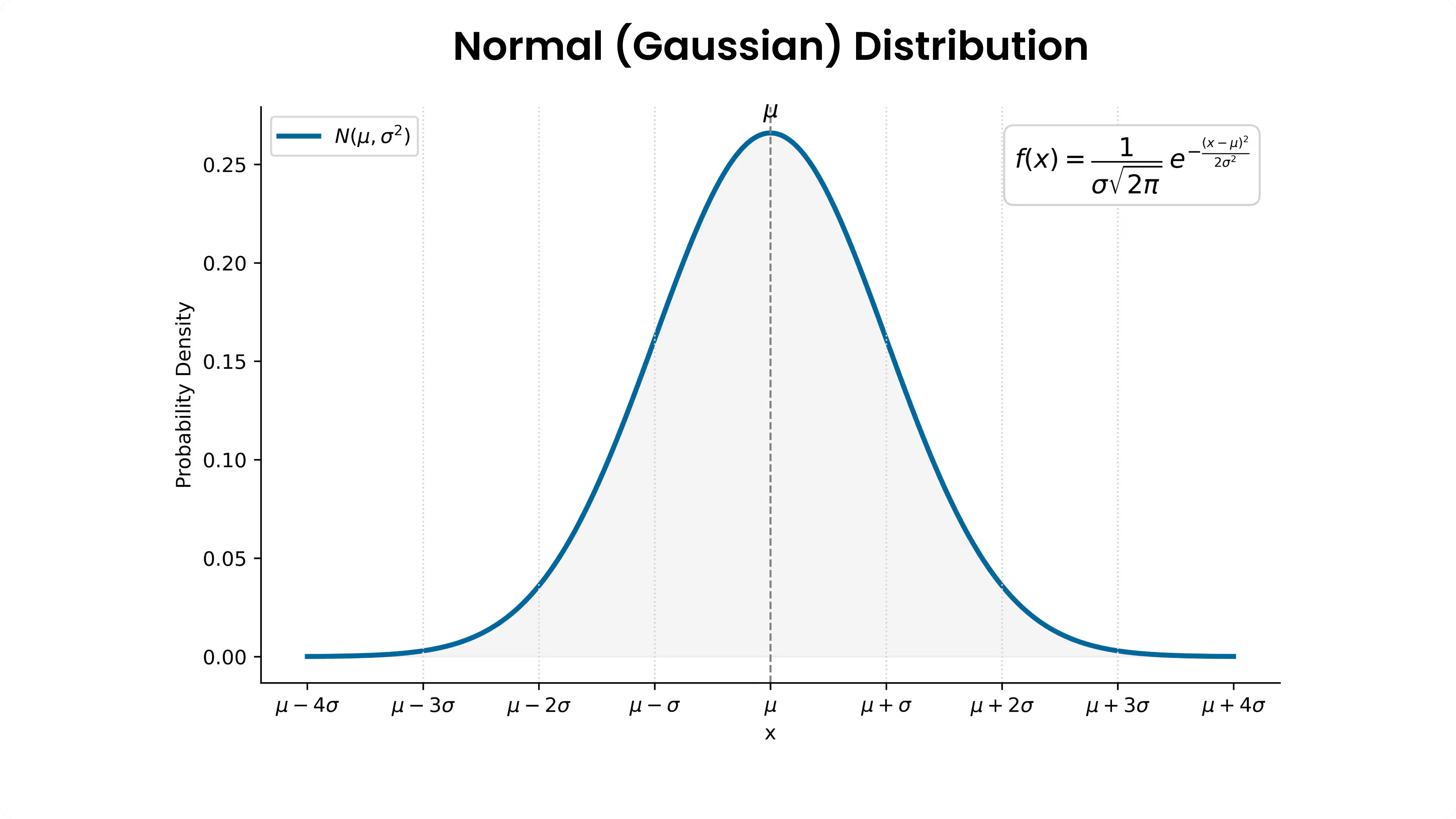
In probability theory and statistics, the normal distribution (also called the Gaussian distribution, or informally the bell curve) is a continuous probability distribution for a real-valued random variable that is perfectly symmetric about its mean. Values close to the mean occur most frequently; values far from the mean occur increasingly rarely, and equally so on both sides. It is one of the most important distributions in statistics: it arises naturally whenever a quantity is the sum of many small, independent effects (see the Central Limit Theorem), it is the distribution with maximum entropy for a given mean and variance, and it underlies most of classical statistical inference. See the formula below for the precise mathematical definition.
A random variable \( X \) that follows a normal distribution is said to be normally distributed and is called a normal deviate. The distribution recurs across many empirical measurements—heights within a population, repeated measurement errors, standardized test scores—a regularity that led Carl Friedrich Gauss and Pierre-Simon Laplace to treat it as the default model for continuous random error (see the history of the distribution).
The Formula
The general form of the probability density function (PDF) of a normal distribution is:
\[ f(x) = \frac{1}{\sigma \sqrt{2\pi}} \, \exp\!\left(-\frac{(x-\mu)^2}{2\sigma^2}\right) \]Here \( \mu \) is the mean (the location parameter, at the center of the curve), \( \sigma \) is the standard deviation (the scale parameter, controlling the spread of the curve), \( e \approx 2.71828 \) is Euler's number, and \( \pi \approx 3.14159 \) is pi. The total area under the curve always equals \( 1 \), since it represents total probability across all outcomes. The two parameters \( \mu \) and \( \sigma \) are all that is needed to fully specify the shape and position of the curve — nothing else about the distribution is left free (see Notation & Parameters below for the constraints each must satisfy).
The exponent \( -(x-\mu)^2/2\sigma^2 \) is a downward-opening parabola in \( x \); exponentiating it produces a peak at \( x = \mu \) that falls off symmetrically and increasingly steeply on both sides. The leading factor \( 1/(\sigma\sqrt{2\pi}) \) is a normalization constant, chosen so that the total area under the curve integrates to \( 1 \).
Notation & Parameters
A normal distribution with mean \( \mu \) and variance \( \sigma^2 \) is written compactly as:
\[ X \sim N(\mu, \sigma^2) \quad \text{or equivalently} \quad X \sim \mathcal{N}(\mu, \sigma^2) \]read as "\( X \) is normally distributed with mean \( \mu \) and variance \( \sigma^2 \)." Several conventions and constraints apply:
- Some sources write the second parameter as \( \sigma \) (standard deviation) instead of \( \sigma^2 \) (variance); the convention in use should be confirmed before values are substituted.
- \( \mu \in \mathbb{R} \) can be any real number: positive, negative, or zero.
- \( \sigma^2 \) must be strictly positive (\( \sigma^2 \in \mathbb{R}_{>0} \)). A distribution with zero variance is not spread out at all — it collapses to a single point, which is modeled using the Dirac delta function rather than a normal density.
- The support of the distribution — the set of values \( X \) can take — is all real numbers, \( x \in \mathbb{R} \), from \( -\infty \) to \( +\infty \). The curve becomes vanishingly thin far from the mean (three standard deviations already cover all but about 0.27% of the total probability, per the empirical rule), so extreme values are possible but increasingly unlikely rather than forbidden.
- An alternative parameterization, used particularly in Bayesian statistics, replaces \( \sigma^2 \) with the precision \( \tau = 1/\sigma^2 \). This simplifies formulas that combine multiple sources of uncertainty, since precisions add directly in a way that variances do not.
Mean & Standard Deviation
Two parameters fully define a normal distribution's shape and position:
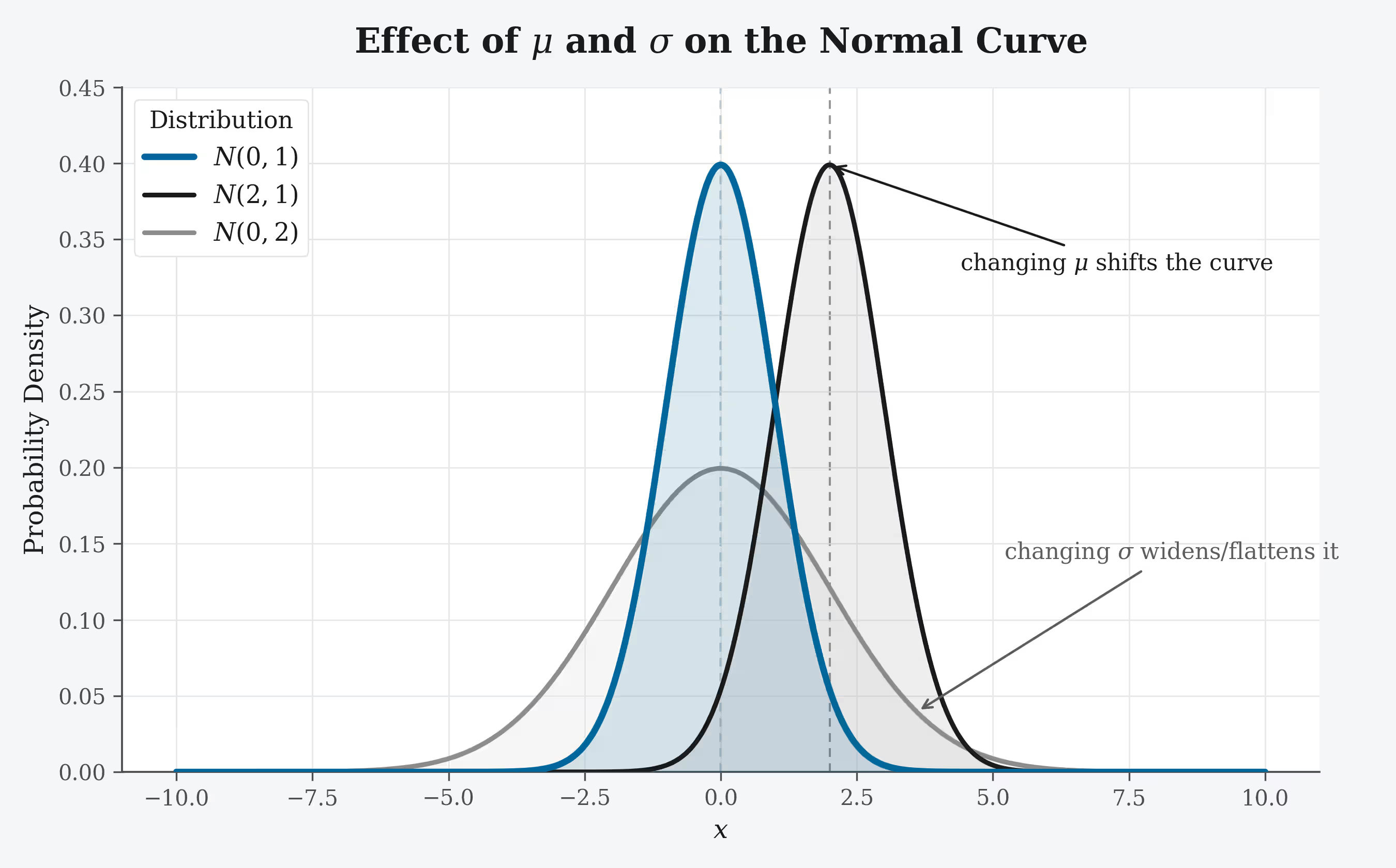
- Mean (\( \mu \)) — the location parameter. It shifts the peak left or right along the x-axis without changing the curve's shape at all. Increasing \( \mu \) slides the whole curve right; decreasing it slides the curve left. Mean, median, and mode all coincide at this single point (see Core Properties).
- Standard deviation (\( \sigma \)) — the scale parameter. It controls how wide or narrow the curve is. A small \( \sigma \) gives a tall, narrow curve (data tightly clustered around the mean); a large \( \sigma \) gives a short, wide curve (data spread out further). Because probability mass is conserved (the area under the curve is always 1), a narrower curve must be taller, and a wider curve must be shorter.
Core Properties
Beyond the formula and its two parameters, the normal distribution has a set of defining mathematical properties that account for its recurrence throughout statistical theory.
Symmetry
The density \( f(x) \) is symmetric about \( x = \mu \): \( f(\mu + a) = f(\mu - a) \) for any \( a \). The shape to the left of \( \mu \) is an exact mirror image of the shape to the right, so the probability of a value falling above the mean equals the probability of falling below it — exactly \( 0.5 \) each.
Mean, Median, and Mode Coincide
Because the curve is both symmetric and unimodal, its three principal measures of central tendency all land on the same point, \( \mu \):
- the mean (the expected value, \( E[X] \)),
- the median (the value splitting the distribution exactly 50/50), and
- the mode (the most probable value, located at the peak of the density).
This is a distinguishing feature: many real-world distributions are skewed, which pulls their mean, median, and mode apart from one another. For the normal distribution, they are always identical.
Variance and Standard Deviation
The variance, \( \operatorname{Var}(X) = \sigma^2 = E[(X-\mu)^2] \), measures the average squared distance of values from the mean. Its square root, \( \sigma \), is the standard deviation, expressed in the same units as the original data and therefore easier to interpret directly. A larger variance means individual observations typically sit farther from the mean.
Skewness
Skewness measures the asymmetry of a distribution. Because the normal distribution is perfectly symmetric, its skewness is exactly:
\[ \text{Skewness} = 0 \]A distribution with a long right tail (such as household income) has positive skew; one with a long left tail has negative skew. A skewness of exactly zero is a defining characteristic of normality and is one of the quantities checked by several normality tests (see the worked example section).
Kurtosis
Kurtosis describes how heavy or light a distribution's tails are relative to its peak. The normal distribution has a kurtosis of:
\[ \text{Kurtosis} = 3, \qquad \text{Excess kurtosis} = 3 - 3 = 0 \]The value \( 3 \) is used as the baseline against which other distributions are measured (their excess kurtosis is reported relative to it). Distributions with heavier tails than normal — more frequent extreme values — are called leptokurtic (positive excess kurtosis, e.g. the Student's t-distribution); those with lighter tails are platykurtic (negative excess kurtosis, e.g. the uniform distribution).
Together, a skewness of \( 0 \) and an excess kurtosis of \( 0 \) are the two most commonly cited numerical signatures used to check whether an empirical dataset is plausibly normal.
Unimodality and Inflection Points
The curve has exactly one peak, located at \( x = \mu \), where the first derivative \( f'(x) = -\dfrac{x-\mu}{\sigma^2}f(x) \) is zero, positive for \( x < \mu \), and negative for \( x > \mu \). A distribution with two or more peaks (bimodal or multimodal) cannot be normal, even if each individual hump looks bell-shaped on its own.
The curve also has exactly two inflection points — the locations where its second derivative changes sign, and the curve switches from curving inward (concave) to curving outward (convex). These sit exactly one standard deviation on either side of the mean:
\[ x = \mu - \sigma \quad \text{and} \quad x = \mu + \sigma \]Visually, this is where the bell's shoulders stop curving toward the peak and begin flattening out toward the tails.
Maximum Entropy
Among all continuous probability distributions with a specified finite mean and variance, the normal distribution is the one with maximum entropy: it is the distribution consistent with a known mean and variance that assumes the least additional structure, spreading probability as evenly as those two constraints allow. This provides a formal, information-theoretic justification for treating the normal distribution as the default model for a variable when only its average and spread are known (see Moments & Generating Functions for the closed-form entropy expression).
Closure Under Linear Combinations
Normal distributions behave predictably under addition and scaling:
- If \( X \sim N(\mu, \sigma^2) \), then \( aX + b \sim N(a\mu + b,\, a^2\sigma^2) \) for any real constants \( a, b \). The family of normal distributions is closed under linear transformations.
- If \( X_1 \sim N(\mu_1, \sigma_1^2) \) and \( X_2 \sim N(\mu_2, \sigma_2^2) \) are independent, then \( X_1 + X_2 \sim N(\mu_1 + \mu_2,\, \sigma_1^2 + \sigma_2^2) \).
- Conversely (Cramér's decomposition theorem), if the sum of two independent random variables is exactly normal, then both variables individually must be normal as well.
This closure property is one reason normal distributions are so convenient to work with analytically, and it directly underlies why sums and averages of many independent quantities tend toward normality (see the Central Limit Theorem).
Moments & Generating Functions
Beyond the mean and variance, distributions are characterized by their full sequence of moments. For a normal distribution, the central moments — \( E[(X-\mu)^p] \) — follow a regular pattern: all odd-order central moments vanish (a consequence of symmetry, discussed under Core Properties), while even-order moments follow a formula involving the double factorial:
| Order \( p \) | Central moment \( E[(X-\mu)^p] \) |
|---|---|
| 0 | \( 1 \) |
| 1 | \( 0 \) |
| 2 | \( \sigma^2 \) (the variance) |
| 3 | \( 0 \) (skewness numerator) |
| 4 | \( 3\sigma^4 \) (kurtosis numerator) |
| 5 | \( 0 \) |
| 6 | \( 15\sigma^6 \) |
The moment generating function (MGF) is a single function that encodes every moment of a distribution at once. For a normal distribution with mean \( \mu \) and variance \( \sigma^2 \), it has an unusually clean closed form:
\[ M(t) = E\left[e^{tX}\right] = \exp\!\left(\mu t + \frac{\sigma^2 t^2}{2}\right) \]Taking the logarithm gives the cumulant generating function, \( g(t) = \ln M(t) = \mu t + \tfrac{1}{2}\sigma^2 t^2 \), a quadratic in \( t \). Because a quadratic polynomial has no terms beyond the second power, the normal distribution is the only distribution whose cumulants beyond the first two (mean and variance) are all exactly zero — it carries no distributional information beyond its mean and variance, which is why it is fully specified by just two parameters.
The related characteristic function, \( \varphi_X(t) = E[e^{itX}] \), always exists (even for distributions whose MGF does not) and for the normal distribution equals \( \varphi_X(t) = \exp(i\mu t - \sigma^2 t^2/2) \). It plays a central role in proving the central limit theorem.
Finally, the differential entropy of a normal distribution — the quantity maximized subject to fixed mean and variance, as noted above — has the closed form:
\[ H(X) = \frac{1}{2}\ln\!\left(2\pi e \, \sigma^2\right) \]The entropy depends only on \( \sigma^2 \), not on \( \mu \): shifting a distribution's location does not change its spread or unpredictability.
Cumulative Distribution Function
The PDF \( f(x) \) (see the formula above) gives the relative likelihood of values near \( x \) but does not itself give a probability — for any continuous distribution, the probability of hitting one exact value is zero. The probability that \( X \) falls at or below some threshold is given instead by the cumulative distribution function (CDF), written \( F(x) \): the area under the PDF curve up to \( x \).
For the standard normal distribution, the CDF is conventionally denoted with the capital Greek letter phi, \( \Phi(z) \), and defined as:
\[ \Phi(z) = \frac{1}{\sqrt{2\pi}} \int_{-\infty}^{z} e^{-t^2/2}\, dt \]This integral has no closed-form elementary antiderivative — it is what mathematicians call a special function — so it must be evaluated numerically or looked up in a table. It is closely related to the error function, \( \operatorname{erf}(x) \), a standard special function defined by:
\[ \operatorname{erf}(x) = \frac{2}{\sqrt{\pi}}\int_0^x e^{-t^2}\,dt, \qquad\text{with}\qquad \Phi(x) = \frac{1}{2}\left[1 + \operatorname{erf}\!\left(\frac{x}{\sqrt{2}}\right)\right] \]For a general normal distribution with mean \( \mu \) and variance \( \sigma^2 \), the CDF reduces to the standard normal CDF via the z-score transform introduced below:
\[ F(x) = \Phi\!\left(\frac{x-\mu}{\sigma}\right) \]The shape of \( \Phi(z) \) is a smooth S-curve (a sigmoid) rising monotonically from 0 to 1:
- \( \Phi(z) \to 0 \) as \( z \to -\infty \) (essentially no probability that far below the mean),
- \( \Phi(0) = 0.5 \) exactly, since half the distribution lies below the mean, and
- \( \Phi(z) \to 1 \) as \( z \to +\infty \) (essentially all probability lies below).
The graph of \( \Phi \) has 2-fold rotational symmetry about the point \( (0, 1/2) \), which gives the identity \( \Phi(-z) = 1 - \Phi(z) \) — the key relationship used to look up negative z-scores from a table built only for positive ones (see the z-table below).
To find the probability that a normal variable \( X \) falls strictly between two values \( a \) and \( b \), subtract the two CDF values:
\[ P(a < X \le b) = F(b) - F(a) = \Phi\!\left(\frac{b-\mu}{\sigma}\right) - \Phi\!\left(\frac{a-\mu}{\sigma}\right) \]The 68–95–99.7 Rule
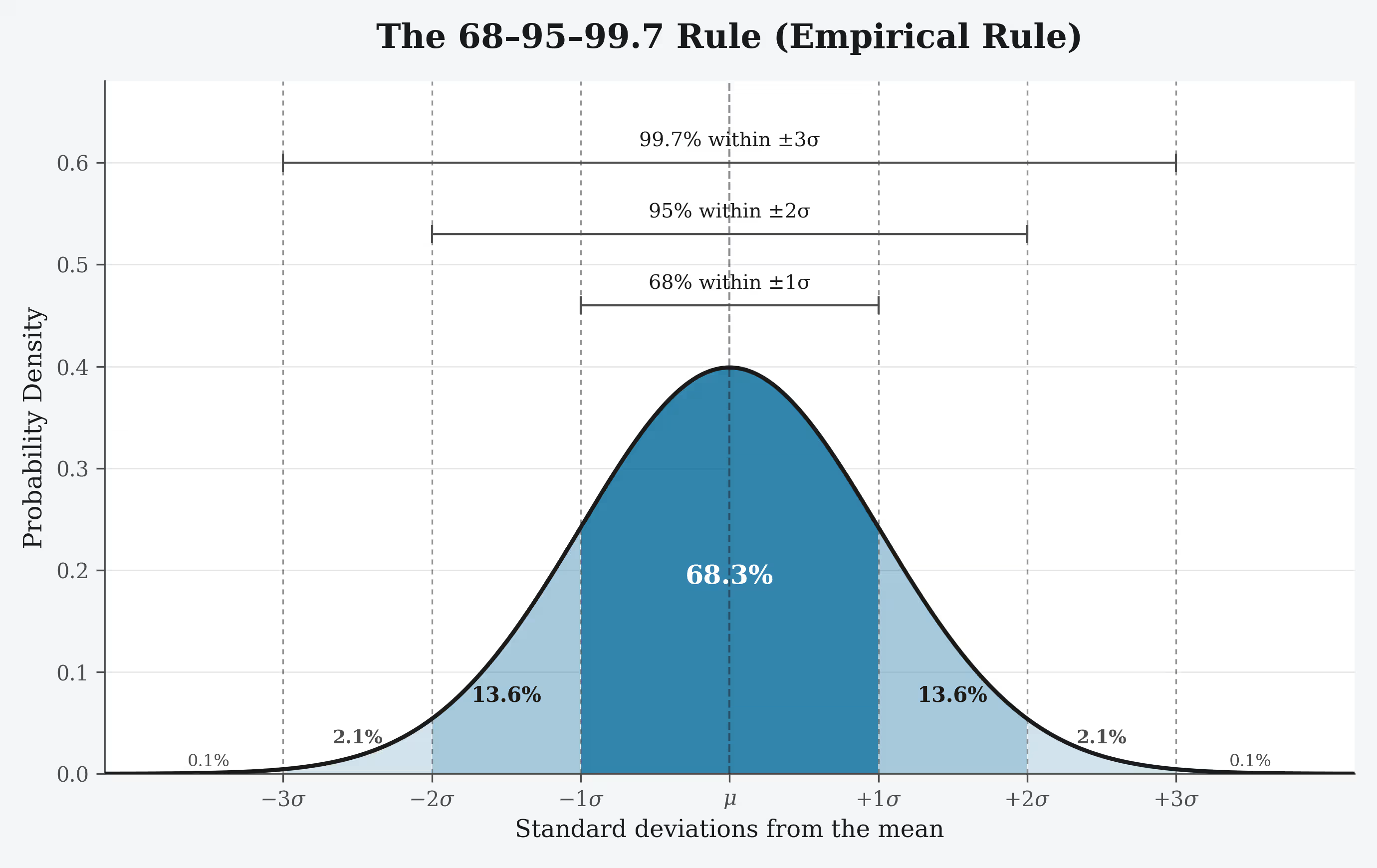
Also called the empirical rule or the three-sigma rule, this describes how probability mass clusters around the mean in any normal distribution, regardless of the specific values of \( \mu \) and \( \sigma \). It follows directly from the cumulative distribution function described above, and is documented in detail by the NIST Engineering Statistics Handbook:
| Range | Approximate probability | Precise probability (12 s.f.) |
|---|---|---|
| \( \mu \pm 1\sigma \) | ~68% | 0.682689492137 |
| \( \mu \pm 2\sigma \) | ~95% | 0.954499736104 |
| \( \mu \pm 3\sigma \) | ~99.7% | 0.997300203937 |
More precisely, the probability that a normal deviate falls within \( n \) standard deviations of the mean is given in terms of the error function by:
\[ P(\mu - n\sigma < X < \mu + n\sigma) = \Phi(n) - \Phi(-n) = \operatorname{erf}\!\left(\frac{n}{\sqrt{2}}\right) \]Values beyond three standard deviations occur with appreciable frequency only in large samples: about 1 in 15,787 observations exceeds \( 4\sigma \), about 1 in 1.74 million exceeds \( 5\sigma \), and about 1 in 506.8 million exceeds \( 6\sigma \) — the threshold used in particle physics to declare a statistically significant discovery. Exact probabilities for any threshold can be read from the standard normal (z) table below.
Standard Normal & Z-Scores
Setting \( \mu = 0 \) and \( \sigma^2 = 1 \) gives the standard normal distribution, written \( N(0,1) \), with density:
\[ \varphi(z) = \frac{1}{\sqrt{2\pi}} e^{-z^2/2} \]This is the simplest case of the normal family, and \( \varphi \) reaches its peak value \( 1/\sqrt{2\pi} \approx 0.3989 \) at \( z=0 \).
Any normal variable \( x \) from a normal distribution \( N(\mu, \sigma^2) \) can be converted to this standard form using the z-score:
\[ z = \frac{x - \mu}{\sigma} \]A z-score expresses how many standard deviations a value sits from the mean — positive if above the mean, negative if below. This allows any two normal distributions, regardless of their own \( \mu \) and \( \sigma \), to be compared on a common scale, and is the basis of the z-table below, which allows probabilities to be looked up without repeating the underlying integral each time.
Going in the reverse direction, if a z-score and the original distribution's parameters are known, the original value can be recovered:
\[ x = \mu + z\sigma \]This standardization also has a probabilistic interpretation: if \( X \sim N(\mu, \sigma^2) \), then \( Z = (X-\mu)/\sigma \) is itself standard normal, \( Z \sim N(0,1) \) — a direct consequence of the closure-under-linear-transformation property discussed in Core Properties.
Standard Normal (Z) Table
A z-table gives the area under the standard normal curve to the left of a given z-score — in other words, \( \Phi(z) \) (see the CDF section above), the probability that a standard normal variable is less than \( z \). To read it: locate the z-score's value to one decimal place along the row, and its second decimal place along the column; the cell where they intersect gives the cumulative probability.
| z | 0.00 | 0.01 | 0.02 | 0.03 | 0.04 | 0.05 |
|---|---|---|---|---|---|---|
| 0.0 | 0.5000 | 0.5040 | 0.5080 | 0.5120 | 0.5160 | 0.5199 |
| 0.5 | 0.6915 | 0.6950 | 0.6985 | 0.7019 | 0.7054 | 0.7088 |
| 1.0 | 0.8413 | 0.8438 | 0.8461 | 0.8485 | 0.8508 | 0.8531 |
| 1.5 | 0.9332 | 0.9345 | 0.9357 | 0.9370 | 0.9382 | 0.9394 |
| 2.0 | 0.9772 | 0.9778 | 0.9783 | 0.9788 | 0.9793 | 0.9798 |
| 2.5 | 0.9938 | 0.9940 | 0.9941 | 0.9943 | 0.9945 | 0.9946 |
| 3.0 | 0.9987 | 0.9987 | 0.9987 | 0.9988 | 0.9988 | 0.9989 |
Certain z-scores are landmark values that recur constantly in applied statistics, particularly in the construction of confidence intervals:
| Confidence level \( p \) | \( z_p \) |
|---|---|
| 90% | 1.645 |
| 95% | 1.960 |
| 98% | 2.326 |
| 99% | 2.576 |
For negative z-scores, use the symmetry identity introduced above: \( \Phi(-z) = 1 - \Phi(z) \). For example, \( \Phi(-1.0) = 1 - 0.8413 = 0.1587 \).
Worked Example
Suppose exam scores in a large class are normally distributed with a mean of \( \mu = 70 \) and a standard deviation of \( \sigma = 10 \). What fraction of students scored above 85?
Step 1 — Standardize: convert the raw score to a z-score.
\[ z = \frac{x - \mu}{\sigma} = \frac{85 - 70}{10} = 1.5 \]Step 2 — Look up \( \Phi(1.5) \): from Table 3, \( \Phi(1.5) = 0.9332 \). This is the probability of scoring at or below 85.
Step 3 — Complement: subtract from 1 to get the probability of scoring above 85.
\[ P(X > 85) = 1 - \Phi(1.5) = 1 - 0.9332 = 0.0668 \]About 6.7% of students scored above 85. The same three steps — standardize, look up, adjust for the tail direction — solve any normal-distribution probability question involving a single threshold; the CDF-subtraction formula from the previous section handles the two-threshold case.
Second question: between what two scores do the middle 95% of students fall? Using \( z_{0.95} = 1.96 \) from Table 4:
\[ x = \mu \pm 1.96\sigma = 70 \pm 1.96(10) = [50.4,\ 89.6] \]Approximately 95% of students scored between about 50 and 90.
The Central Limit Theorem
The normal distribution's pervasiveness does not stem from individual measurements being normal, but from the fact that sums and averages of measurements tend toward normality, largely independent of how the original measurements are distributed. The central limit theorem (CLT) is the formal statement of this fact.
Let \( X_1, X_2, \ldots, X_n \) be independent and identically distributed random variables with finite mean \( 0 \) and finite variance \( \sigma^2 \) (any starting distribution works, not just normal ones), and define the scaled sample mean:
\[ Z = \sqrt{n}\left(\frac{1}{n}\sum_{i=1}^{n} X_i\right) \]Then, as \( n \to \infty \), the probability distribution of \( Z \) converges to \( N(0, \sigma^2) \) — regardless of the shape of the original distribution the \( X_i \) were drawn from, provided it has finite mean and variance. The theorem does not require the effects to act additively forever; a moderately large sample size (often \( n \gtrsim 30 \) as a rule of thumb, though this depends on how skewed the original distribution is) is often enough for the approximation to be useful in practice.
This explains why the normal distribution is such a common approximation for other distributions under the right conditions:
- the binomial distribution \( B(n,p) \) is approximately \( N(np,\, np(1-p)) \) for large \( n \) when \( p \) is not too close to 0 or 1;
- the Poisson distribution with rate \( \lambda \) is approximately \( N(\lambda, \lambda) \) for large \( \lambda \);
- the chi-squared distribution \( \chi^2(k) \) is approximately \( N(k, 2k) \) for large degrees of freedom \( k \) (see Related Distributions); and
- the Student's t-distribution converges to \( N(0,1) \) as its degrees of freedom grow (also covered under Related Distributions).
The approximation tends to be least accurate in the tails of the distribution, which is why more careful analysis (or an exact distribution, where available) is preferred when small tail probabilities matter.
Estimating Parameters from Data
The true population parameters \( \mu \) and \( \sigma \) are rarely known and must typically be estimated from a sample. Given \( n \) independent observations \( x_1, x_2, \ldots, x_n \) drawn from \( N(\mu, \sigma^2) \):
Sample Mean
The sample mean is the standard estimator of \( \mu \):
\[ \bar{x} = \frac{1}{n}\sum_{i=1}^{n} x_i \]By the Lehmann–Scheffé theorem, \( \bar{x} \) is the uniformly minimum-variance unbiased estimator of \( \mu \). In finite samples it is itself exactly normally distributed:
\[ \bar{x} \sim N\!\left(\mu, \frac{\sigma^2}{n}\right) \]Its standard deviation, \( \sigma/\sqrt{n} \), is called the standard error of the mean. Because it shrinks with \( \sqrt{n} \) rather than \( n \), halving the standard error requires quadrupling the sample size, a relationship used to plan sample sizes for opinion polls and Monte Carlo simulations.
Sample Variance
The sample variance, using Bessel's correction (dividing by \( n-1 \) rather than \( n \) to make the estimator unbiased), is:
\[ s^2 = \frac{1}{n-1}\sum_{i=1}^{n} (x_i - \bar{x})^2 \]Its square root, \( s \), is the sample standard deviation. The \( (n-1) \) divisor exists because computing \( \bar{x} \) from the same sample "uses up" one degree of freedom; dividing by \( n \) instead would systematically underestimate the true variance.
Confidence Intervals
By Cochran's theorem, for normally distributed data the sample mean \( \bar{x} \) and sample variance \( s^2 \) are statistically independent. This independence is what allows the construction of the t-statistic:
\[ t = \frac{\bar{x} - \mu}{s/\sqrt{n}} \sim t_{n-1} \]which follows a Student's t-distribution with \( n-1 \) degrees of freedom (see Related Distributions). Inverting this relationship gives a confidence interval for the unknown \( \mu \). For large samples, the t-distribution converges to normal, and a common approximate 95% confidence interval is:
\[ \mu \in \left[\bar{x} - 1.96\frac{s}{\sqrt{n}},\ \ \bar{x} + 1.96\frac{s}{\sqrt{n}}\right] \]meaning that if the sampling process were repeated many times, about 95% of the intervals constructed this way would contain the true population mean \( \mu \). For small samples, the exact t-distribution quantile should be used instead of \( 1.96 \), since it correctly accounts for the extra uncertainty introduced by estimating \( \sigma \) from a limited sample.
Generating Normal Random Numbers
Computers natively generate uniform random numbers — every value in a range equally likely — rather than normal ones, so simulations and machine learning code require a method to transform uniform randomness into normally distributed randomness. Established approaches include:
- Inverse transform sampling — draw a uniform random number \( u \) on \( (0,1) \), then apply the inverse of the CDF, \( z = \Phi^{-1}(u) \), to obtain a standard normal value. Conceptually the simplest method, though \( \Phi^{-1} \) (the probit function) has no closed form and must itself be approximated numerically to high precision.
- Box–Muller transform — takes two independent uniform random numbers \( U, V \) on \( (0,1) \) and combines them into two independent standard normal values at once: \[ X = \sqrt{-2\ln U}\,\cos(2\pi V), \qquad Y = \sqrt{-2\ln U}\,\sin(2\pi V) \] This works because, for a bivariate normal vector \( (X,Y) \), the squared norm \( X^2+Y^2 \) follows an exponential distribution and the angle is uniform around the circle — both of which are easy to sample directly.
- Ziggurat algorithm — a faster, still-exact rejection-sampling method widely used in production numerical libraries, since it avoids the transcendental function calls that Box–Muller requires in the common case.
These methods are rarely implemented by hand in practice: libraries such as NumPy (numpy.random.normal()) or PyTorch (torch.randn()) handle the conversion internally, using variants of the methods above. The conversion nonetheless occurs under the hood any time code requests "random Gaussian noise."
A Short History
The normal distribution's roots trace to Abraham de Moivre, who in 1733 derived it as an approximation to the binomial distribution while studying coin-flip probabilities, publishing the result formally in 1738. De Moivre did not, however, articulate anything resembling a modern probability density function — his result was framed purely as an approximation to binomial coefficients.
It was Carl Friedrich Gauss who, in his 1809 work Theoria Motus Corporum Coelestium, gave the distribution its enduring association with his name. Gauss used it to model measurement errors in astronomical observations, and in the process introduced the method of least squares and the method of maximum likelihood — deriving the normal law as the unique distribution of errors under which the arithmetic mean is the most probable estimate of an unknown quantity.
Pierre-Simon Laplace made independent and foundational contributions: he first posed the general problem of aggregating multiple observations in 1774, calculated the key normalizing integral \( \int e^{-t^2}\,dt = \sqrt{\pi} \) in 1782, and in 1810 proved and presented the fundamental central limit theorem to the French Academy, cementing the distribution's theoretical importance well beyond its original use in astronomy.
Later in the 19th century, James Clerk Maxwell showed the distribution was not merely a convenient mathematical fiction but occurs directly in physical nature, using it to describe the velocity distribution of gas particles — a cornerstone of the kinetic theory of gases.
The name "normal distribution" itself gained currency later still, popularized near the turn of the 20th century largely through the work of the statistician Karl Pearson. Pearson himself later expressed some regret over the name, noting it risked implying that other distributions were somehow "abnormal" — a connotation not intended by the original coinage, which referred to the normal equations used in fitting the curve, with "normal" in its older, technical sense of "orthogonal," not "typical."
Where It Shows Up
The occurrence of the normal distribution in practical problems falls loosely into a few categories: exact physical laws that happen to be Gaussian, approximate laws justified by the central limit theorem, distributions assumed to be normal as a maximum-entropy default, and cases arising after systematic effects are modeled out (as in regression residuals). A selection of concrete examples across each category:
- Feature scaling — z-score normalization is a standard preprocessing step before training many machine learning models.
- Anomaly detection — points many standard deviations from the mean are flagged as statistical outliers.
- Gaussian Mixture Models — unsupervised clustering via weighted combinations of several normal distributions.
- Generative AI — diffusion models generate images by iteratively adding and then learning to remove Gaussian noise.
- Standardized testing — scores such as the SAT are scaled to approximate a target normal distribution (historically, mean 500 and standard deviation 100 per section).
- Measurement error — errors in physical experiments are conventionally modeled as normal, since it is the most conservative assumption consistent with a known mean and variance.
- Quality control — manufacturing tolerances typically assume normally distributed variation to set acceptable limits (a common origin of "Six Sigma" methodology).
- Physics — the ground-state wavefunction of the quantum harmonic oscillator and the velocity distribution of particles in an ideal gas (Maxwell–Boltzmann statistics) are both exactly Gaussian in form.
- Hypothesis testing — t-tests, ANOVA, and most classical significance tests rest on an assumption of underlying normality, whether exact or approximate via the central limit theorem.
Normal distributions are sometimes misapplied to data that is not well approximated by them. Heavy-tailed financial returns are a documented example where normal assumptions have historically underestimated the risk of extreme events. When outliers or heavy tails are expected, distributions built for that purpose, such as the Student's t or a log-Lévy model, are generally more appropriate.
Frequently Asked Questions
- It is a symmetric, bell-shaped probability distribution where values near the mean occur most often and values far from the mean occur rarely, in equal proportion on both sides.
- Also called the 68-95-99.7 rule, it states that about 68% of data falls within 1 standard deviation of the mean, about 95% within 2 standard deviations, and about 99.7% within 3 standard deviations.
- The standard normal distribution is a special case of the normal distribution with mean 0 and standard deviation 1. Any normal variable can be converted to it using the z-score transform, z = (x - mu) / sigma.
- It is used in feature scaling (z-score normalization), as a prior in Bayesian models, for anomaly detection, in Gaussian mixture models, and as the noise model in diffusion-based generative AI.
- A normal distribution has a skewness of 0, since it is perfectly symmetric, and a kurtosis of 3 (equivalently, an excess kurtosis of 0), which serves as the baseline for comparing the tail-heaviness of other distributions.
- A z-table gives the area under the standard normal curve to the left of a given z-score. Find the z-score's first two digits in the row and its second decimal in the column; the number where they meet is the cumulative probability.
- It says that if you repeatedly take random samples and average them, those averages will form a roughly normal distribution, even if the original data was not normal, as long as the sample size is reasonably large.
- The chi-squared distribution arises from summing squared standard normal variables, the Student's t-distribution approximates the normal distribution for small samples with unknown variance, and the log-normal distribution describes variables whose logarithm is normally distributed.