Hypergeometric Distribution

What Is a Hypergeometric Distribution?

In probability theory and statistics, the hypergeometric distribution is the discrete probability distribution of the number of successes obtained when drawing a fixed number \( n \) of items, without replacement, from a finite population of size \( N \) that contains a known number \( K \) of successes (and \( N-K \) failures). Each draw removes an item permanently from the population, so the composition of what remains - and therefore the probability of success on the next draw - shifts with every draw already made. See the formula below for the precise mathematical definition.

The hypergeometric distribution is the natural sibling of the binomial distribution: both count successes across a fixed number of draws from a two-outcome population, but the binomial distribution assumes sampling with replacement (or an effectively infinite population), while the hypergeometric distribution captures what actually happens when the population is finite and items are not put back. This single difference - replacement or not - is responsible for every structural difference between the two distributions explored in this article, from their variance formulas (see Core Properties) to when one can stand in for the other (see Binomial & Normal Approximations).

The Formula

The probability mass function (PMF) of a hypergeometric distribution, which gives the probability of observing exactly \( k \) successes among \( n \) draws made without replacement, is:

where \( \binom{K}{k} \) counts the number of ways to choose \( k \) successes from the \( K \) available in the population, \( \binom{N-K}{n-k} \) counts the number of ways to choose the remaining \( n-k \) draws as failures from the \( N-K \) failures available, and \( \binom{N}{n} \) is the total number of equally likely ways to choose any \( n \) items from the full population of \( N \). The PMF is therefore a direct application of the classical (equally likely outcomes) definition of probability: favorable combinations divided by total combinations.

Unlike the binomial PMF, no fixed success probability \( p \) appears anywhere in the formula - the entire dependence on how "success-heavy" the population is comes through the counts \( N \), \( K \), and \( n \) themselves. The support of \( k \) is also not simply \( \{0, 1, \ldots, n\} \) as in the binomial case; it is restricted to

since there cannot be more successes drawn than either the sample size \( n \) or the number of successes \( K \) available, and there cannot be so few successes that the remaining draws would need more failures than the \( N-K \) failures actually present.

Notation & Parameters

A hypergeometric distribution with population size \( N \), \( K \) successes in that population, and sample size \( n \) is written compactly as:

read as "\( X \) follows a hypergeometric distribution with population \( N \), \( K \) successes, and sample size \( n \)." Three parameters, all non-negative integers, fully specify the distribution:

• \( N \) is the population size - the total number of items available to draw from, \( N \ge 1 \).
• \( K \) is the number of successes in the population, \( 0 \le K \le N \); the remaining \( N-K \) items are failures.
• \( n \) is the sample size - the fixed number of items drawn without replacement, \( 0 \le n \le N \).
• The support of the distribution is the finite integer range \( \max(0, n-(N-K)) \le k \le \min(n, K) \) described in The Formula, which can be narrower than \( \{0,\ldots,n\} \) whenever the population does not contain enough successes or failures to fill every draw either way.
• Some sources define the parameters symmetrically as \( (N, n, K) \) or use \( m \) in place of \( K \); the underlying quantities are identical, but it is worth checking a source's convention before matching formulas against software output.
• The defining assumption is sampling without replacement from a fixed, finite population: once an item is drawn it is not returned, so successive draws are not independent, in direct contrast to the binomial distribution's i.i.d. trials.

Core Properties

Every descriptive property of the hypergeometric distribution can be compared directly against its binomial counterpart with \( p = K/N \), since the two distributions describe the same underlying experiment differing only in whether draws are replaced.

Mean (Expected Value)

The expected value of a hypergeometric random variable has exactly the same form as the binomial mean, with the population proportion of successes \( K/N \) standing in for \( p \):

This identity holds regardless of replacement because expectation is linear: each individual draw, considered marginally (before conditioning on the outcomes of the other draws), is exactly as likely to be a success as picking one item uniformly at random from the population, namely with probability \( K/N \).

Variance

The variance is where sampling without replacement leaves its clearest fingerprint. It matches the binomial variance formula but is scaled down by an extra factor:

The final term, \( \dfrac{N-n}{N-1} \), is the finite population correction factor, and it is always \( \le 1 \) for \( n \ge 1 \). It formalizes the intuition that removing items without replacement makes later draws less independently random than draws made with replacement - the population "remembers" what has already been taken out, which mechanically suppresses variability compared to the binomial case. As \( N \to \infty \) with \( K/N \) and \( n \) fixed, the correction factor tends to \( 1 \) and the hypergeometric variance converges to the binomial variance \( np(1-p) \) (see Binomial & Normal Approximations).

Skewness

Skewness measures the asymmetry of a distribution. For a hypergeometric distribution it is:

The distribution is exactly symmetric whenever \( K = N/2 \) or \( n = N/2 \) - that is, when successes make up exactly half the population, or exactly half the population is drawn - since either condition makes the numerator vanish. Away from those special cases, the sign of \( (N-2K) \) and \( (N-2n) \) together determines whether the distribution leans left or right.

Kurtosis

Kurtosis describes the shape of a distribution's tails relative to its center. The hypergeometric excess kurtosis has a considerably more involved closed form than the binomial's, reflecting the extra dependence introduced by the three interacting parameters \( N \), \( K \), and \( n \); in practice it is computed numerically from software rather than by hand, and, as with skewness, it converges to the corresponding binomial excess kurtosis as \( N \to \infty \) with \( K/N \) and \( n \) held fixed.

Mode

The mode - the most probable number of successes - is given by \( \left\lfloor \dfrac{(n+1)(K+1)}{N+2} \right\rfloor \), a formula that closely parallels the binomial mode's \( \lfloor (n+1)p \rfloor \) once \( K/N \) is substituted for \( p \) and the small "\( +1, +2 \)" adjustments from the finite, hypergeometric setting are accounted for.

Shape as N, K and n Vary

With three interacting parameters instead of the binomial's two, the hypergeometric PMF's shape depends on how \( N \), \( K \), and \( n \) move both individually and relative to one another.

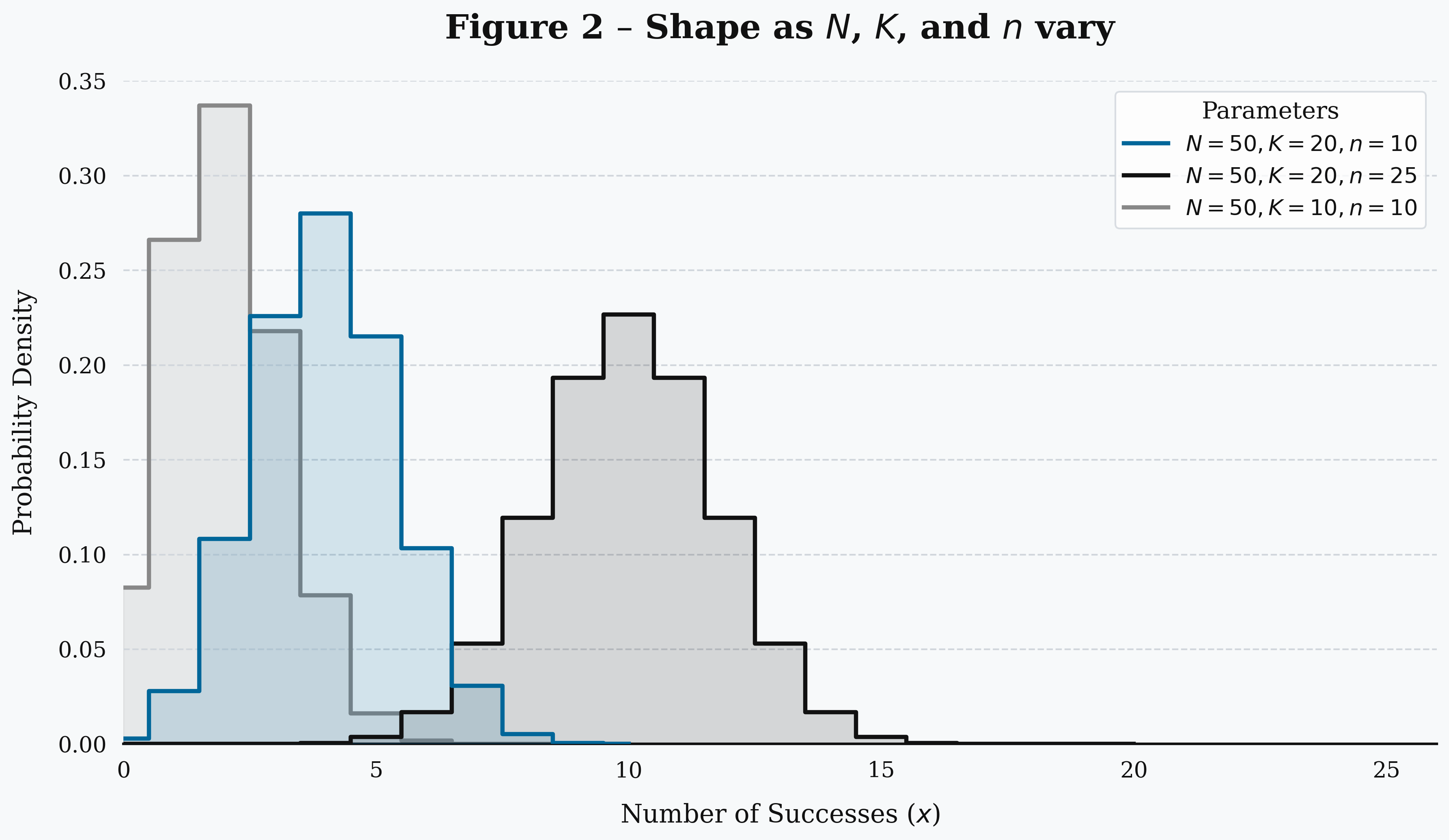
• Increasing the success proportion \( K/N \) with \( n \) fixed shifts the distribution's mass to the right, exactly as increasing \( p \) does for the binomial distribution, per the mean formula \( E[X] = nK/N \) above.
• Increasing the sample size \( n \) with \( N \) and \( K/N \) fixed spreads the distribution over a wider range of possible success counts, though the finite population correction ensures this spread grows more slowly than it would under binomial sampling.
• Increasing the population size \( N \) with \( K/N \) and \( n \) fixed pushes the finite population correction \( (N-n)/(N-1) \) toward \( 1 \), making the shape converge visibly toward the corresponding binomial PMF - the essence of the binomial approximation below.
• When \( n \) is close to \( N \) - a large fraction of the population is sampled - the distribution narrows sharply, since with so few items left undrawn, the final count of successes is nearly determined by \( K \) and \( n \) alone.

Moments & Generating Functions

The moment generating function (MGF) of a hypergeometric random variable can be written in closed form using the generalized hypergeometric function \( {}_2F_1 \) - the special function that gives the distribution its name:

Unlike the binomial or negative binomial MGFs, this expression does not factor into a simple power of a single-trial term, precisely because the draws are not independent - the dependence between draws is what breaks the "product of identical pieces" structure seen in i.i.d. sampling. In practice, the mean and variance in Core Properties are derived far more directly by treating \( X \) as a sum of dependent indicator variables (one per draw) than by differentiating this MGF.

The corresponding probability generating function takes the analogous form \( G(z) = E[z^X] = \dfrac{\binom{N-K}{n}}{\binom{N}{n}}\, {}_2F_1(-n,-K;N-K-n+1;z) \), and both functions are used chiefly in theoretical derivations and combinatorial identities rather than routine calculation.

Cumulative Distribution Function

The cumulative distribution function (CDF), \( F(k) = P(X \le k) \), gives the probability that a hypergeometric variable takes a value at or below a given threshold. It is obtained by summing the PMF over every valid success count up to \( k \):

Because the support is the finite range described in The Formula, the hypergeometric CDF is a staircase with a jump at every integer in that range, starting at \( 0 \) below the lower bound and reaching exactly \( 1 \) at the upper bound, mirroring the finite, bounded shape of the binomial CDF rather than the negative binomial's unbounded staircase. Statistical software evaluates \( F(k) \) directly from cumulative sums of binomial coefficients rather than requiring a closed-form special-function expression.

Worked Example

Suppose a shipment contains \( N = 40 \) electronic components, of which \( K = 6 \) are defective and the remaining \( 34 \) are good. A quality inspector selects \( n = 5 \) components at random, without replacement, for testing. Let \( X \sim \operatorname{Hypergeometric}(40, 6, 5) \) denote the number of defective components among the five selected. What are the mean and standard deviation of \( X \), and what is the probability that exactly two of the five selected components are defective?

Step 1 - Mean: using \( E[X] = nK/N \) from Core Properties:

Step 2 - Variance and standard deviation: using \( \operatorname{Var}(X) = n\dfrac{K}{N}\!\left(1-\dfrac{K}{N}\right)\dfrac{N-n}{N-1} \):

Step 3 - Probability of exactly two defective components: using the PMF with \( k=2 \):

There is roughly a 13.6% chance that exactly two of the five tested components turn out defective. Because the expected count is only \( 0.75 \), observing two defectives is somewhat above average but far from implausible - a useful sanity check the inspector might run before deciding whether the sample suggests the whole shipment should be rejected.

Estimating Parameters from Data

In most applications, the population size \( N \) and sample size \( n \) are known by design - they describe the physical sampling procedure itself - leaving only the number of successes \( K \) in the population as genuinely uncertain. Given an observed count of successes \( X = k \) in a sample of size \( n \), the natural maximum likelihood estimator of \( K \) is:

This estimator arises from finding the integer \( K \) that maximizes the PMF for the observed \( k \), and it underlies classical capture-recapture methods for estimating an unknown population total: if \( K \) marked individuals are released into a population of unknown size \( N \), and a later sample of size \( n \) recaptures \( k \) marked individuals, the same relationship can be inverted to estimate \( N \) itself.

When the hypergeometric distribution is used the other way - to test whether an observed count of successes in a sample is consistent with a hypothesized \( K \), rather than to estimate \( K \) from data - the relevant tool is Fisher's exact test, which computes exact hypergeometric tail probabilities to assess association in small, finite \( 2\times2 \) contingency tables where the normal or chi-squared approximations used for large samples are unreliable.

Binomial & Normal Approximations

Two approximations to the hypergeometric distribution are commonly used, one that recovers a much simpler distribution when the population is large, and one that applies when the sample size itself is large.

Binomial Limit

When the population size \( N \) is much larger than the sample size \( n \) - a common rule of thumb is \( n/N < 0.05 \) or, more conservatively, \( n/N < 0.1 \) - each draw removes only a negligible fraction of the population, so the changing composition that defines sampling without replacement barely matters in practice. In this regime, the hypergeometric distribution is well approximated by a binomial distribution with matching sample size and success probability:

This is precisely why opinion polls and quality-control samples drawn from very large populations are routinely analyzed with binomial - rather than hypergeometric - formulas: the finite population correction factor from Core Properties is close enough to \( 1 \) that the distinction is immaterial for practical purposes.

Normal Approximation

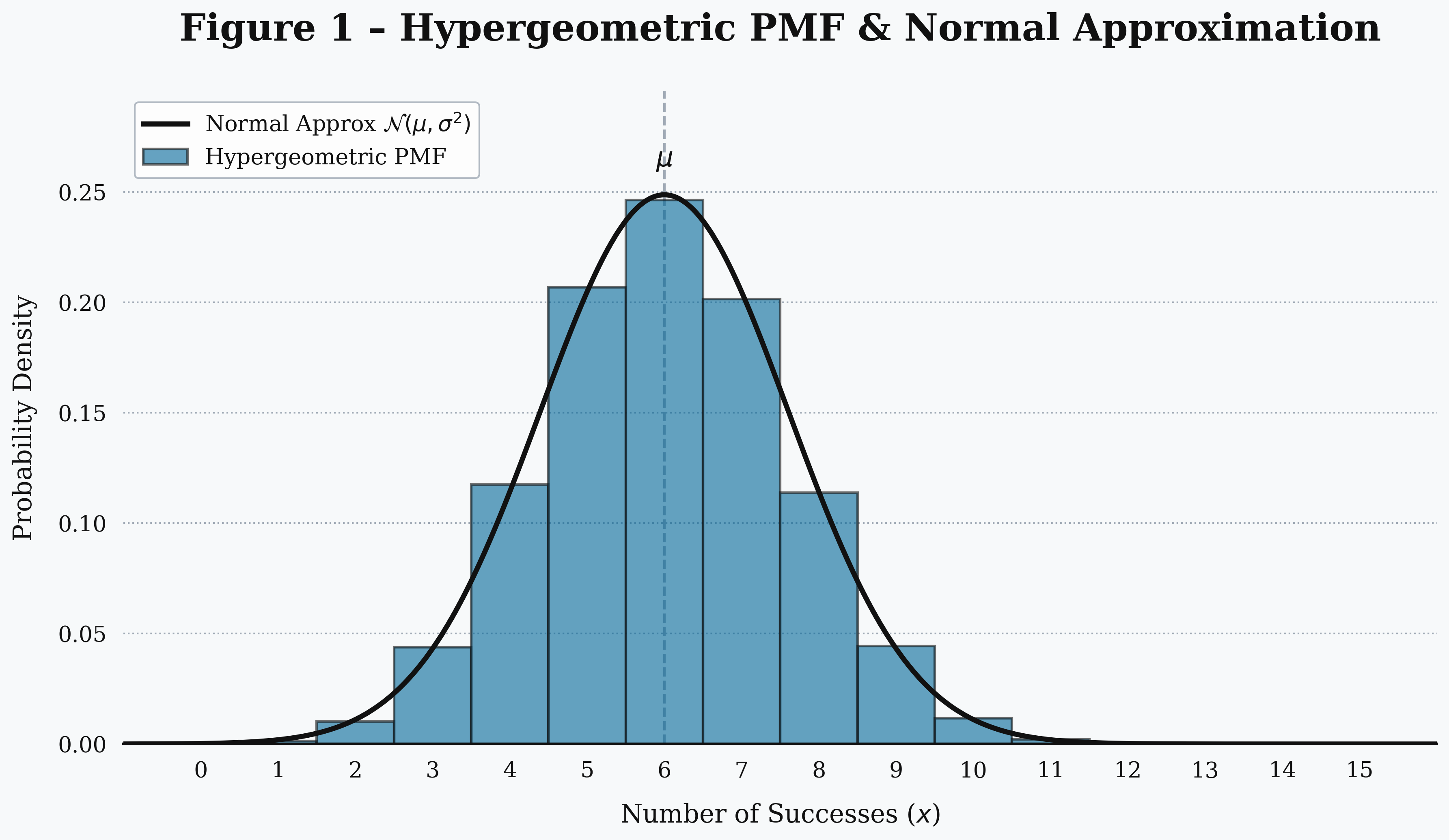
When the sample size \( n \) is reasonably large (and \( N \) is not simultaneously so much larger that the binomial approximation above already applies more simply), the central limit theorem justifies approximating a hypergeometric random variable as approximately normal, with the exact hypergeometric mean and variance:

As with the binomial normal approximation, a continuity correction of \( \pm 0.5 \) improves accuracy, and the approximation works best when the hypergeometric mean is not too close to either edge of its finite support.

Multivariate Hypergeometric

The ordinary hypergeometric distribution assumes exactly two categories in the population - success and failure. The multivariate hypergeometric distribution generalizes this to any number \( c \) of categories: a population of size \( N \) is partitioned into \( c \) groups of sizes \( K_1, K_2, \ldots, K_c \) (with \( K_1+\cdots+K_c = N \)), and a sample of size \( n \) is drawn without replacement. The probability of drawing exactly \( k_1 \) items from category 1, \( k_2 \) from category 2, and so on, is:

Setting \( c=2 \) recovers the ordinary two-category hypergeometric PMF from The Formula exactly, with \( K_1=K \) and \( K_2=N-K \). A classic example is drawing a hand of cards from a standard deck and tracking how many cards of each of the four suits appear - a direct multivariate hypergeometric setup with \( c=4 \) categories of \( K_i=13 \) cards each.

Related Distributions

The hypergeometric distribution sits alongside several closely related distributions, each obtained by varying one of its defining assumptions:

• Binomial distribution - the distribution obtained when sampling with replacement instead of without; the limiting case of the hypergeometric distribution as \( N \to \infty \) with \( K/N \) fixed (see Binomial & Normal Approximations).
• Multivariate hypergeometric distribution - the generalization to more than two categories in the population, described in Multivariate Hypergeometric above.
• Negative hypergeometric distribution - the waiting-time counterpart that counts the number of failures drawn, without replacement, before a fixed number of successes is reached, directly paralleling how the negative binomial distribution relates to the binomial.
• Normal distribution - the limiting distribution of a (standardized) hypergeometric variable as the sample size \( n \) grows large, a consequence of the central limit theorem for sampling without replacement.
• Beta-binomial distribution - shares the hypergeometric distribution's property of overdispersion relative to the binomial, though it arises from a different mechanism (a random success probability rather than sampling without replacement).

Generating Hypergeometric Random Numbers

Because the hypergeometric distribution models an explicit finite-population sampling process, one direct way to generate a draw is to simulate the population and the sampling procedure itself:

1. Represent the population as \( K \) success items and \( N-K \) failure items.
2. Draw \( n \) items uniformly at random from the population, one at a time, removing each drawn item before the next draw (sampling without replacement).
3. Return \( X \), the count of success items among the \( n \) drawn, as the hypergeometric draw.

This direct simulation works but becomes inefficient for large \( N \). Statistical software instead typically uses specialized algorithms - such as inverse-transform sampling on the PMF, or rejection-based methods tuned for the hypergeometric case - that avoid explicitly representing the full population.

In practice, these details are handled internally: for example, NumPy's numpy.random.hypergeometric(ngood, nbad, nsample) and SciPy's scipy.stats.hypergeom.rvs(M, n, N) both return draws from a Hypergeometric\( (N, K, n) \) distribution without requiring the underlying population or sampling procedure to be implemented by hand.

A Short History

The hypergeometric distribution's roots lie in some of the earliest problems in enumerative combinatorics - counting favorable outcomes among equally likely arrangements - applied to games of chance involving drawing objects (cards, balls, lots) from a fixed collection without returning them. Problems of this flavor appear in the work of the same seventeenth- and eighteenth-century probabilists who laid the groundwork for the binomial distribution, with the "urn model" - drawing colored balls from an urn without replacement - becoming the standard illustrative device still used to teach the distribution today.

The distribution's name derives from its connection to the hypergeometric function, a special function studied extensively in the eighteenth and nineteenth centuries by mathematicians including Euler and Gauss; the probabilities in the distribution's PMF sum according to identities governed by this same function (see Moments & Generating Functions). The distribution's role in formal statistical inference solidified in the twentieth century through Ronald Fisher's development of the exact test for \( 2\times2 \) contingency tables that bears his name (see Estimating Parameters from Data), which remains one of the distribution's most widely used modern applications.

Where It Shows Up

Any scenario involving a fixed number of draws made without replacement from a finite, known population is, in principle, hypergeometric. A selection of concrete examples across statistics, quality control, and everyday probability:

• Quality control and acceptance sampling - inspecting a fixed number of items from a finite production lot for defects, exactly as in the worked example above, is a textbook hypergeometric application in manufacturing.
• Card games and lotteries - the number of a particular suit, rank, or set of winning numbers drawn in a hand of cards or a lottery draw is hypergeometric by construction, since cards and lottery balls are drawn without replacement from a fixed, known set.
• Ecology - capture-recapture population estimation - estimating an unknown population size by marking, releasing, and later resampling individuals relies directly on hypergeometric probabilities, as described in Estimating Parameters from Data.
• Fisher's exact test in statistics - testing for association between two binary variables in a small \( 2\times2 \) contingency table uses exact hypergeometric tail probabilities rather than large-sample approximations.
• Auditing and sampling from finite records - selecting a sample of transactions, invoices, or records from a finite, known population to estimate an error rate is a standard hypergeometric setting in financial and compliance auditing.
• Genetics and bioinformatics - testing whether a gene set is unexpectedly enriched among a sample of genes drawn from a fixed background gene list (gene set enrichment analysis) reduces to a hypergeometric probability calculation.
• Committee and lottery selection problems - the number of members from a specific subgroup selected when choosing a fixed-size committee at random from a larger group, without replacement, is a direct hypergeometric calculation.

As with the binomial distribution, the hypergeometric model can be misapplied when the population is not actually fixed and finite in the way assumed - for instance, when items are effectively replaced or when the population composition changes for reasons other than the sampling itself - in which case a binomial or other model may be more appropriate instead (see Related Distributions).

Frequently Asked Questions

• What is a hypergeometric distribution in simple terms? +
  It is the probability distribution of the number of successes obtained when drawing a fixed number of items, without replacement, from a finite population that contains a known number of successes and a known number of failures.
• What is the difference between a hypergeometric distribution and a binomial distribution? +
  A binomial distribution assumes draws are made with replacement (or from an effectively infinite population), so the success probability stays constant across trials. A hypergeometric distribution draws without replacement from a finite population, so the success probability changes after each draw because the population composition shifts.
• What are the mean and variance of a hypergeometric distribution? +
  For a hypergeometric random variable X counting successes in n draws without replacement from a population of size N containing K successes, the mean is E[X] = nK/N and the variance is Var(X) = n(K/N)(1-K/N)((N-n)/(N-1)). The final factor, (N-n)/(N-1), is the finite population correction and has no counterpart in the binomial variance.
• When can a binomial distribution approximate a hypergeometric distribution? +
  When the population size N is much larger than the sample size n (a common rule of thumb is n/N less than about 0.05 or 0.1), each draw only negligibly changes the remaining composition, so the hypergeometric distribution is well approximated by a binomial distribution with p = K/N.
• Why does the hypergeometric distribution have smaller variance than the binomial for the same n and p? +
  Sampling without replacement removes successes and failures from the population as draws are made, which mechanically reduces the randomness in later draws compared to sampling with replacement. This is captured exactly by the finite population correction factor (N-n)/(N-1), which is always less than or equal to 1.
• Is the hypergeometric distribution discrete or continuous? +
  It is discrete: the random variable counts a whole number of successes and can only take integer values within a bounded range determined by the population size, sample size, and number of successes available, so probability is described by a probability mass function.
• What is the multivariate hypergeometric distribution? +
  It is the generalization of the hypergeometric distribution to a population with more than two categories - for example, drawing colored balls from an urn containing several colors rather than just successes and failures - and it reduces exactly to the ordinary hypergeometric distribution when there are only two categories.
• What distributions are related to the hypergeometric distribution? +
  The binomial distribution approximates the hypergeometric distribution when the population is large relative to the sample, the multivariate hypergeometric distribution generalizes it to more than two categories, the negative hypergeometric distribution asks the complementary waiting-time question, and the normal distribution approximates it for large sample sizes via the central limit theorem.