
Artificial Neural Networks (ANN)
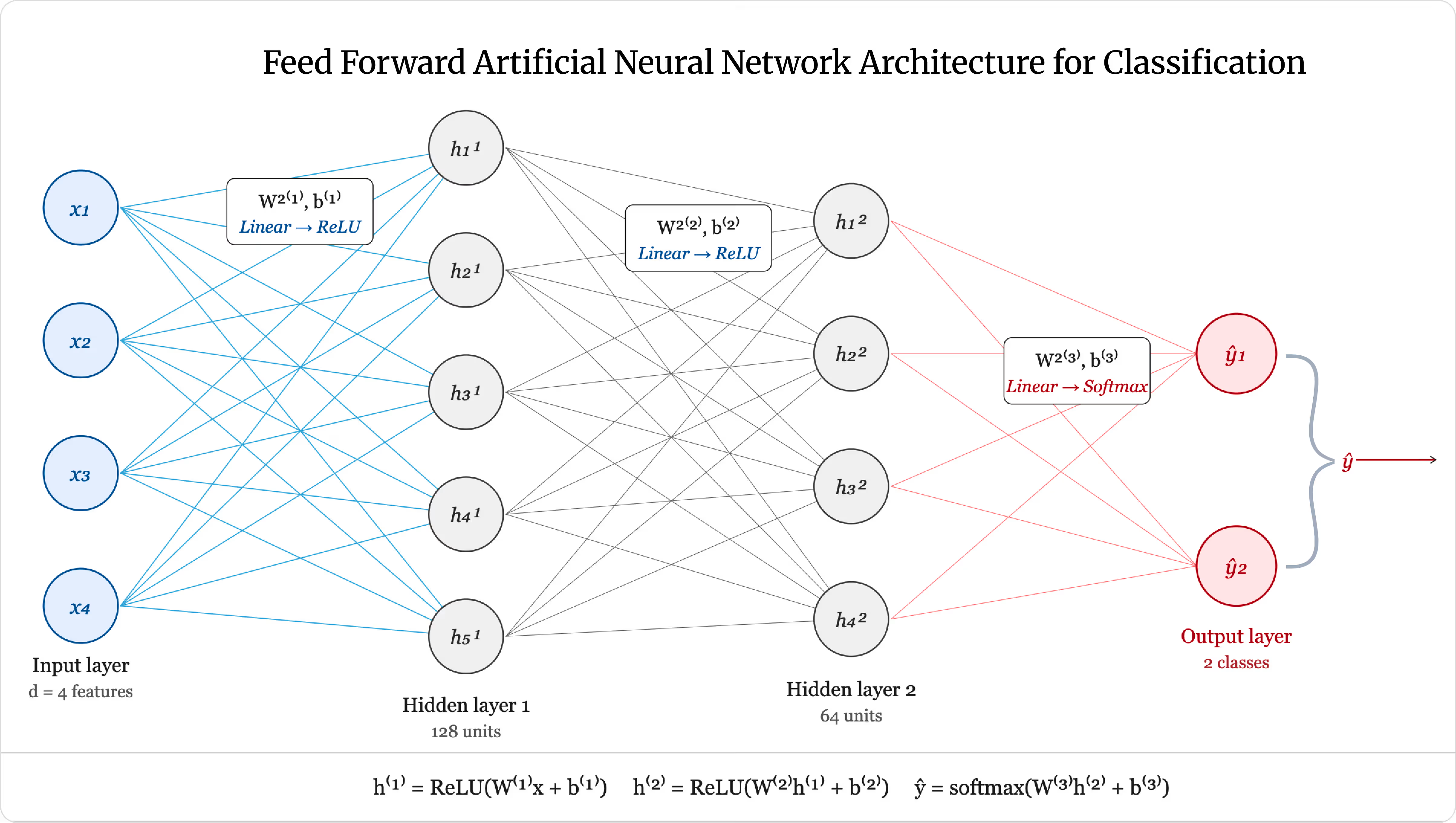
Abstract
This guide provides a complete, textbook-depth treatment of Artificial Neural Networks (ANN)-from the biological inspiration and historical origins through the full mathematics of forward propagation, backpropagation, gradient-based optimization, and regularization. It surveys the major architecture families (feedforward networks, MLPs, CNNs, RNNs, LSTM/GRU, and Transformers), compares activation and loss functions, walks through a complete training pipeline, and includes from-scratch Python and PyTorch implementations, worked numerical examples, and a rigorous comparison of ANN against machine learning, deep learning, and the perceptron.
Introduction
An Artificial Neural Network (ANN) is a computing system made of layers of interconnected artificial neurons, loosely modeled on the biological brain, that learns to map inputs to outputs by adjusting the numeric weight of every connection through repeated exposure to data. ANNs are the architectural foundation beneath image recognition, machine translation, voice assistants, self-driving perception systems, and large language models-in short, beneath essentially every branch of modern deep learning.
Where ANNs are used: computer vision, natural language processing, speech recognition, recommendation engines, fraud detection, medical diagnosis, autonomous vehicles, and generative AI all rely on some variant of an ANN. Why they matter: unlike hand-coded rules, an ANN learns its own internal representation of a problem directly from data, which is what allows the same underlying technique to scale from recognizing handwritten digits to powering a modern language model.
| Definition | A layered network of artificial neurons that learns weighted connections from data via backpropagation and gradient descent. |
| Invented by | Warren McCulloch & Walter Pitts (1943 model); Frank Rosenblatt (1958 perceptron); Rumelhart, Hinton & Williams (1986 backpropagation) |
| First paper | "A Logical Calculus of the Ideas Immanent in Nervous Activity" (McCulloch & Pitts, 1943) |
| Main applications | Computer vision, NLP, speech recognition, recommendation systems, autonomous driving, generative AI |
| Advantages | Learns complex non-linear patterns automatically; generalizes across images, text, audio, and tabular data; improves with more data and compute |
| Limitations | Needs large labeled datasets; computationally expensive to train; acts as a "black box" with limited interpretability; prone to overfitting without regularization |
| Common architectures | Feedforward (FNN), MLP, CNN, RNN, LSTM/GRU, Transformer |
This guide takes you from that one-sentence definition to full practical fluency. We cover the biological inspiration and historical origins of the field, build up the complete mathematics of how a network computes and learns, tour the major architecture families used in production systems today, and finish with real-world applications, common pitfalls, and a clear-eyed comparison of ANN against related terms that are frequently-and often incorrectly-used interchangeably: machine learning, deep learning, and the perceptron.
By the end of this article you will be able to explain how an ANN computes a prediction and learns from error, derive backpropagation from first principles, choose appropriate activation and loss functions for a given problem, recognize the major architecture families and when to use each, implement a working network in Python and PyTorch, and precisely distinguish ANN from machine learning, deep learning, and the perceptron.
What is an Artificial Neural Network?
An Artificial Neural Network is a computational model composed of layers of simple processing units called artificial neurons (or nodes), connected to one another by weighted links. Each neuron receives one or more inputs, combines them using learned weights and a bias term, applies a non-linear activation function, and passes its output forward to the next layer. Collectively, this layered structure allows the network to approximate extremely complex functions-mapping raw inputs (pixels, words, sensor readings, tabular features) to useful outputs (classifications, numeric predictions, sequences of text).
Formally, an ANN can be viewed as a parameterized function \( f_{\theta}: \mathbb{R}^n \to \mathbb{R}^m \) that maps an input vector to an output vector, where \( \theta \) represents every weight and bias in the network. "Training" a neural network means searching for values of \( \theta \) that make \( f_{\theta} \) fit a training dataset well, using an iterative optimization procedure rather than hand-coded rules.
Three properties define what makes a model an ANN rather than some other kind of machine learning algorithm:
- Layered composition: neurons are organized into layers, and information generally flows from an input layer, through one or more hidden layers, to an output layer.
- Learned weighted connections: the strength of every connection is a numeric weight that is adjusted during training, rather than fixed by a human designer.
- Non-linear activation: each neuron applies a non-linear function to its weighted input, which is what allows the network, as a whole, to represent non-linear relationships in data.
A single artificial neuron in isolation-just weights, a bias, and an activation function-is exactly the computational unit described in our companion article on the perceptron. An ANN is what you get when you connect many such units into a network of layers, replace the perceptron's non-differentiable step function with a smooth activation function, and train the whole system jointly using backpropagation.
Biological Neuron vs Artificial Neuron
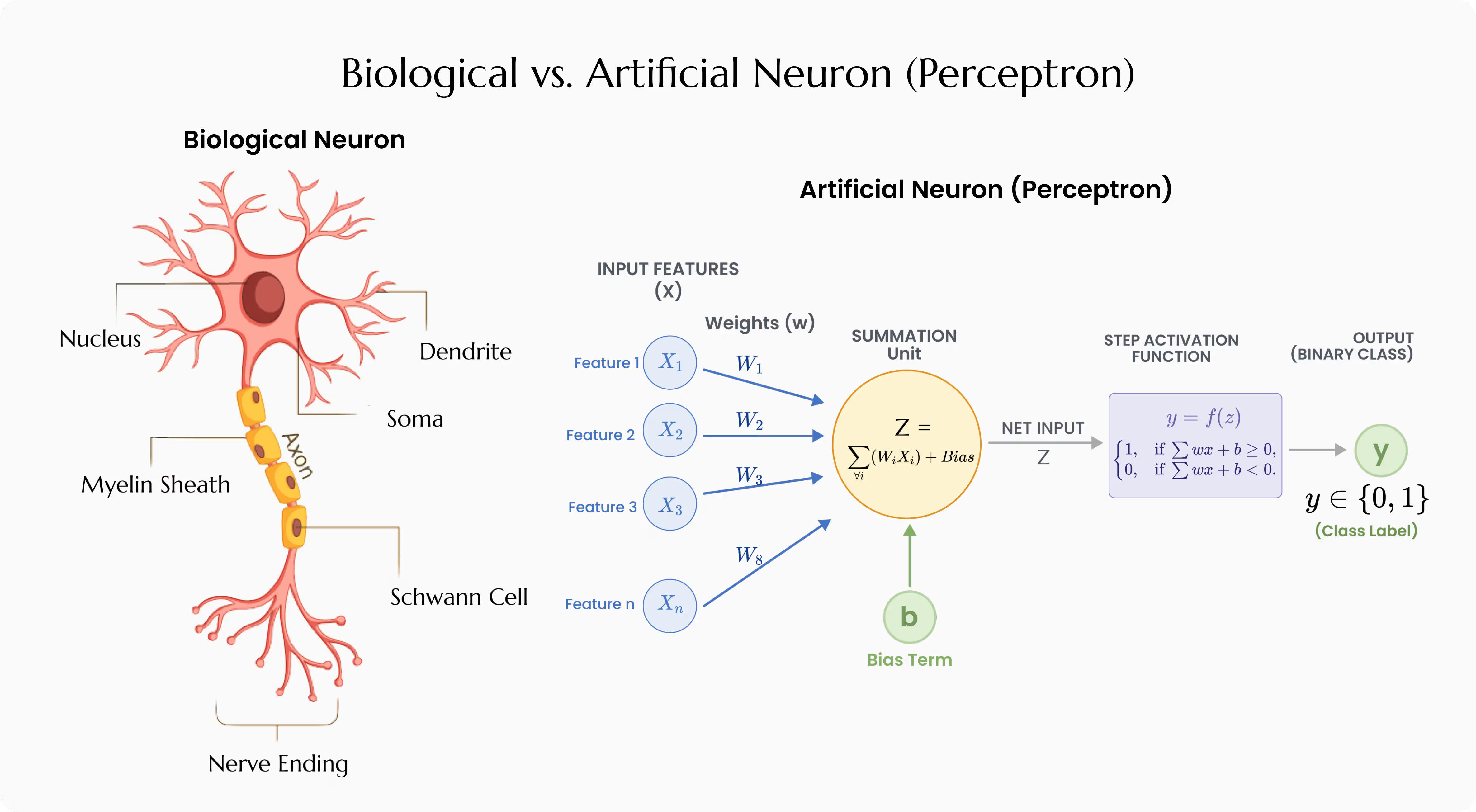
The artificial neuron borrows its name and a loose structural analogy from biology, but the two systems differ enormously in mechanism, scale, and learning process. Understanding both the similarity and the difference prevents two common mistakes: dismissing ANNs as "just like the brain" (they are not) and dismissing the analogy entirely as meaningless (it is a useful and historically important abstraction).
| Aspect | Biological Neuron | Artificial Neuron |
|---|---|---|
| Input | Electrochemical signals via dendrites from other neurons | Numeric values \( x_1, \ldots, x_n \) from data or previous layer |
| Signal strength | Synaptic strength, modified by neurotransmitter release | Numeric weight \( w_i \), adjusted by gradient descent |
| Integration | Soma sums incoming electrical potentials | Weighted sum \( z = \sum w_i x_i + b \) |
| Firing decision | All-or-nothing action potential if threshold exceeded | Smooth activation function (sigmoid, tanh, ReLU, etc.) |
| Output transmission | Electrical pulse propagated along the axon | Numeric output value passed to next layer |
| Learning mechanism | Synaptic plasticity (e.g., long-term potentiation), poorly understood in detail | Backpropagation and gradient-based weight updates, fully specified mathematically |
| Scale | ~86 billion neurons, ~100 trillion synapses in a human brain | Modern large models: billions of parameters; still orders of magnitude below the brain's connectivity |
| Energy efficiency | Roughly 20 watts for the entire brain | Large models require kilowatts to megawatts of power for training |
Note. Neuroscientists generally caution against over-interpreting the analogy. Real biological learning involves neurotransmitters, glial cells, structural rewiring, and mechanisms that have no equivalent in an ANN's backpropagation-based training. The artificial neuron is best understood as an engineering abstraction inspired by biology, not a faithful simulation of it.
Components of an Artificial Neural Network
Every ANN, regardless of how deep or specialized, is built from the same small set of components.
Neurons (Nodes)
The basic processing unit. Each neuron receives inputs, computes a weighted sum plus bias, and applies an activation function to produce its output.
Weights
Numeric parameters attached to every connection between neurons. Weights determine how strongly the output of one neuron influences the input of the next, and they are the primary quantity adjusted during training.
Bias
An additional learnable parameter added to each neuron's weighted sum, allowing the neuron's activation threshold to shift independently of its inputs-analogous to the intercept term in a linear equation.
Layers
- Input layer: receives the raw feature values; it performs no computation of its own.
- Hidden layer(s): intermediate layers that transform the input into increasingly useful internal representations. A network with more than one hidden layer is commonly called a "deep" network.
- Output layer: produces the network's final prediction, shaped to match the task (a single value for regression, a probability distribution over classes for classification, etc.).
Activation Function
A non-linear function applied to each neuron's weighted sum. Covered in full detail in Activation Functions.
Loss Function
A function that quantifies how far the network's predictions are from the true target values. Training is, at its core, the process of minimizing this function. Covered in Loss Functions.
Optimizer
The algorithm that updates weights and biases to reduce the loss, using gradients computed via backpropagation. Covered in Gradient Descent and Optimizers.
Learning Rate
A hyperparameter controlling how large a step the optimizer takes with each weight update. Too high and training becomes unstable; too low and training becomes impractically slow.
How ANN Works: Step by Step
At a high level, training and using an ANN follows the same repeating loop regardless of architecture:
- Initialize the network's weights and biases, typically with small random values (see Weight Initialization).
- Forward propagation: feed an input example through the network, layer by layer, to produce a prediction.
- Compute loss: compare the prediction to the true target using a loss function.
- Backpropagation: compute the gradient of the loss with respect to every weight and bias in the network, using the chain rule.
- Update parameters: adjust every weight and bias in the direction that reduces the loss, scaled by the learning rate, via an optimizer such as gradient descent or Adam.
- Repeat steps 2-5 for many examples and many passes (epochs) over the dataset until the loss stops improving meaningfully or a stopping criterion is met.
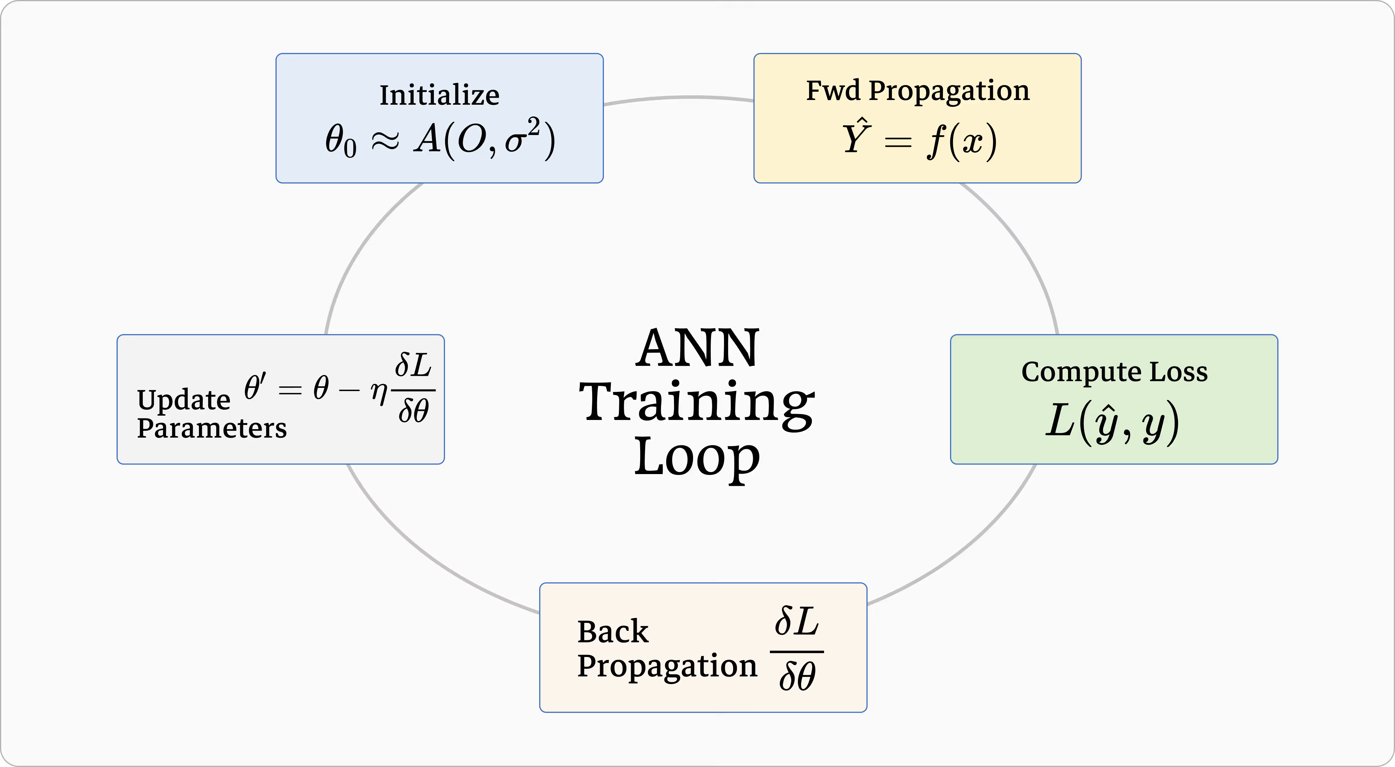
Once trained, using the network for prediction (often called inference) requires only step 2-forward propagation-with the final learned weights held fixed.
Tip. It helps to think of training as search: the network's weights define a point in a very high-dimensional space, the loss function defines a landscape over that space, and training is the process of walking downhill toward a point with low loss, guided at every step by the gradient computed through backpropagation.
Network Architecture
"Architecture" refers to how neurons are organized and connected-the number of layers, the number of neurons per layer, and the pattern of connections between them. Architecture choices have a large effect on what a network can learn efficiently.
Fully Connected (Dense) Layers
In a fully connected layer, every neuron is connected to every neuron in the previous layer. This is the default, most general-purpose layer type, used in the classic Multilayer Perceptron and as the final decision-making layers in most other architectures.
Depth and Width
A network's depth is its number of layers; its width is the number of neurons in a given layer. Increasing depth allows the network to compose simpler features into more abstract ones across successive layers; increasing width allows each layer to capture a larger number of distinct patterns. Both increase representational capacity, but also increase the risk of overfitting and the computational cost of training.
Universal Approximation
The Universal Approximation Theorem, first established for sigmoidal activation functions by Cybenko (1989) and later generalized to broader classes of networks, states that a feedforward network with a single hidden layer containing a finite number of neurons, using a suitable non-linear activation function, can approximate any continuous function on a compact input domain to arbitrary accuracy, given enough neurons in that layer.
Warning. This theorem is frequently misunderstood as saying "one hidden layer is always enough in practice." It only guarantees that a sufficiently wide single-layer network exists-it says nothing about how many neurons that requires, nor whether such a network is learnable through gradient descent from a realistic amount of training data. In practice, deeper networks with moderate width are usually far easier to train and require far fewer total parameters than a single extremely wide layer.
Research Perspective. A separate line of theoretical work-often grouped under the heading of depth efficiency-shows that some functions expressible by a moderately deep network would require an exponentially wider shallow network to approximate to the same accuracy. This helps explain, in a more formal way than intuition alone, why practitioners consistently favor moderate depth over extreme width even though both routes are covered by the same existence guarantee.
Connection Patterns Beyond Fully Connected
Not every architecture connects every neuron to every other neuron. Convolutional layers restrict connections to local spatial regions and share weights across positions; recurrent layers add connections that loop back in time; attention-based layers compute connection strength dynamically based on content rather than fixed position. These specialized connection patterns are the subject of the next section.
Types of Neural Networks
"Artificial Neural Network" is an umbrella term. In practice, almost every production system uses one of a handful of specialized architecture families, each suited to a particular kind of data.
Feedforward Neural Networks (FNN)
A Feedforward Neural Network is the simplest ANN architecture: information moves in exactly one direction, from input to output, with no cycles or loops. Every layer feeds forward into the next, never back. This is the base pattern that all other architectures either follow directly or extend.
Multilayer Perceptrons (MLP)
A Multilayer Perceptron is a feedforward network with one or more fully connected hidden layers between the input and output, each using a non-linear activation function. Despite the name, an MLP's neurons are not classical perceptrons with a step function-they use smooth activations and are trained with backpropagation, not the perceptron learning rule. The MLP is the direct historical successor to the perceptron and the architecture that first proved that stacking layers overcomes the linear-separability limitation described in our perceptron article.
MLPs remain a strong default choice for structured, tabular data-spreadsheet-style datasets with a fixed number of numeric or categorical features per example.
Convolutional Neural Networks (CNN)
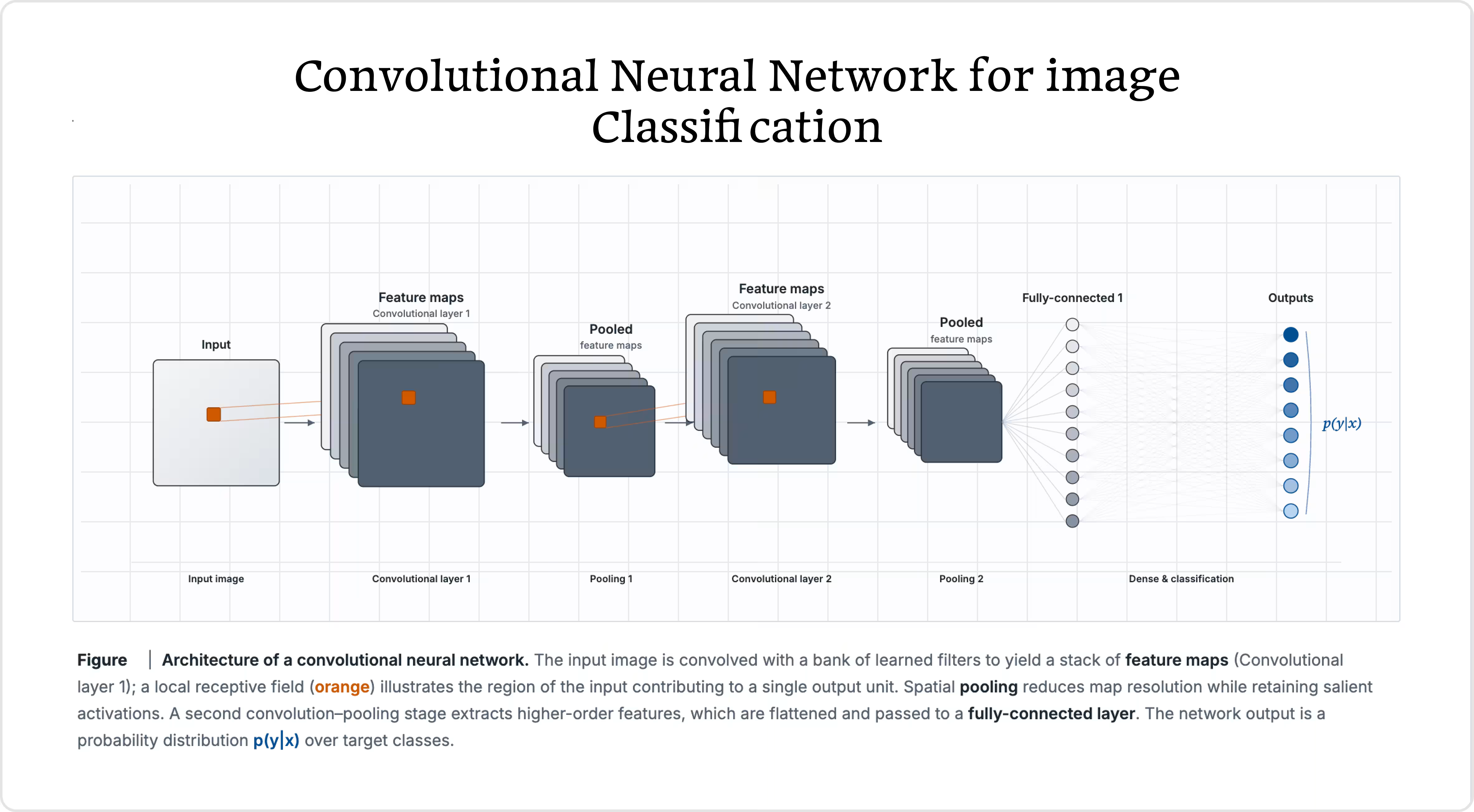
A Convolutional Neural Network is designed for data with strong spatial structure, most commonly images. Instead of fully connecting every input pixel to every neuron, a CNN applies small learnable filters (kernels) that slide across the input, detecting local patterns such as edges, textures, and shapes. The same filter weights are reused across every spatial position-a property called weight sharing-which dramatically reduces the number of parameters compared to a fully connected layer operating on raw pixels.
- Convolutional layers: apply learnable filters to extract local features.
- Pooling layers: downsample feature maps (e.g., max pooling), reducing spatial size and providing a degree of translation invariance.
- Fully connected layers: typically appear near the end of the network to combine extracted features into a final prediction.
CNNs power the vast majority of modern computer vision systems, including image classification, object detection, medical image analysis, and facial recognition.
Recurrent Neural Networks (RNN)
A Recurrent Neural Network is designed for sequential data-text, time series, audio-where the order of elements carries meaning. Unlike a feedforward network, an RNN maintains a hidden state that is updated at every time step and fed back into the network alongside the next input, giving it a form of memory of what it has seen so far.
\[ h_t = \tanh(W_{xh} x_t + W_{hh} h_{t-1} + b_h) \]where \( x_t \) is the input at time step \( t \), \( h_{t-1} \) is the hidden state carried over from the previous step, and \( h_t \) is the updated hidden state. This recurrence is what allows an RNN to process sequences of arbitrary length with a fixed number of parameters.
Warning. Plain (vanilla) RNNs suffer badly from the vanishing gradient problem: when backpropagating error through many time steps, gradients are repeatedly multiplied by values less than one, shrinking exponentially and making it very difficult to learn dependencies that span long sequences. This limitation directly motivated LSTM and GRU.
LSTM and GRU
Long Short-Term Memory (LSTM) networks, introduced by Hochreiter and Schmidhuber in 1997, solve the vanishing gradient problem by adding a separate cell state that acts as a long-term memory conveyor belt, along with three learned gates-input, forget, and output-that control what information is added to, removed from, and read out of that memory at each time step. Because the cell state's update is largely additive rather than repeatedly multiplicative, gradients can flow across many time steps without vanishing as quickly.
The Gated Recurrent Unit (GRU), introduced later, simplifies the LSTM design by merging the cell state into the hidden state and reducing three gates to two (update and reset). GRUs are computationally cheaper and often perform comparably to LSTMs, making them a popular lighter-weight alternative.
| Property | Vanilla RNN | LSTM | GRU |
|---|---|---|---|
| Gates | None | Input, forget, output | Update, reset |
| Long-range dependency handling | Poor | Strong | Strong |
| Parameter count | Lowest | Highest | Moderate |
| Training speed | Fastest | Slowest | Faster than LSTM |
Transformer-Based Neural Networks
The Transformer, introduced in the 2017 paper "Attention Is All You Need," replaces recurrence entirely with a mechanism called self-attention, which lets every position in a sequence directly attend to every other position in a single step, regardless of distance. This solves the long-range dependency problem more directly than LSTM/GRU and, crucially, allows the entire sequence to be processed in parallel during training rather than one time step at a time-a major practical advantage on modern GPU and TPU hardware.
Transformers are the architecture behind essentially all modern large language models, and are increasingly used for vision (Vision Transformers), audio, and multimodal tasks as well.
Research Perspective. Standard self-attention compares every position in a sequence with every other position, so its computational and memory cost grows quadratically with sequence length-a significant practical limitation as context windows extend into the hundreds of thousands of tokens. This has motivated an active research area around sparse, linear, and windowed attention variants, as well as state-space models, that aim to preserve the parallelizable, long-range strengths of the Transformer while reducing this quadratic cost.
| Architecture | Best Suited For | Key Structural Idea |
|---|---|---|
| Feedforward / MLP | Tabular / structured data | Fully connected layers, one-directional flow |
| CNN | Images, spatial data | Local receptive fields, weight sharing |
| RNN | Short sequences | Recurrent hidden state carried across time steps |
| LSTM / GRU | Longer sequences, time series | Gated memory cells that resist vanishing gradients |
| Transformer | Language, large-scale sequence & multimodal tasks | Self-attention across all positions, parallelizable |
Activation Functions
An activation function is applied to the weighted sum \( z \) of every neuron to introduce non-linearity. Without it, no matter how many layers a network has, the entire model would collapse into a single linear transformation, since a composition of linear functions is itself linear-a network with a thousand linear layers would be no more expressive than one.
Sigmoid
\[ \sigma(z) = \frac{1}{1 + e^{-z}}, \quad \sigma(z) \in (0, 1) \]Squashes any real number into the range \( (0, 1) \), making it useful for binary classification output layers where the output is interpreted as a probability. Its major drawback is saturation: for large positive or negative \( z \), the gradient of sigmoid approaches zero, which slows or stalls learning in deep networks-a key contributor to the vanishing gradient problem.
Tanh
\[ \tanh(z) = \frac{e^{z} - e^{-z}}{e^{z} + e^{-z}}, \quad \tanh(z) \in (-1, 1) \]Similar to sigmoid but zero-centered, which often makes optimization better behaved. It still saturates at the extremes and shares the same vanishing-gradient weakness.
ReLU (Rectified Linear Unit)
\[ \text{ReLU}(z) = \max(0, z) \]The most widely used activation function in modern hidden layers. It is computationally cheap, does not saturate for positive inputs, and empirically leads to faster convergence than sigmoid or tanh in deep networks. Its drawback is the dying ReLU problem: a neuron whose weighted input is consistently negative outputs zero and receives zero gradient, effectively becoming permanently inactive.
Leaky ReLU
\[ \text{LeakyReLU}(z) = \begin{cases} z & z \geq 0 \\ \alpha z & z < 0 \end{cases}, \quad \alpha \text{ typically } 0.01 \]Addresses the dying ReLU problem by allowing a small, non-zero gradient when the input is negative, keeping the neuron "alive."
Softmax
\[ \text{softmax}(z)_i = \frac{e^{z_i}}{\sum_{j=1}^{K} e^{z_j}} \]Converts a vector of \( K \) raw scores (logits) into a probability distribution that sums to 1. It is almost exclusively used in the output layer of multi-class classification networks.
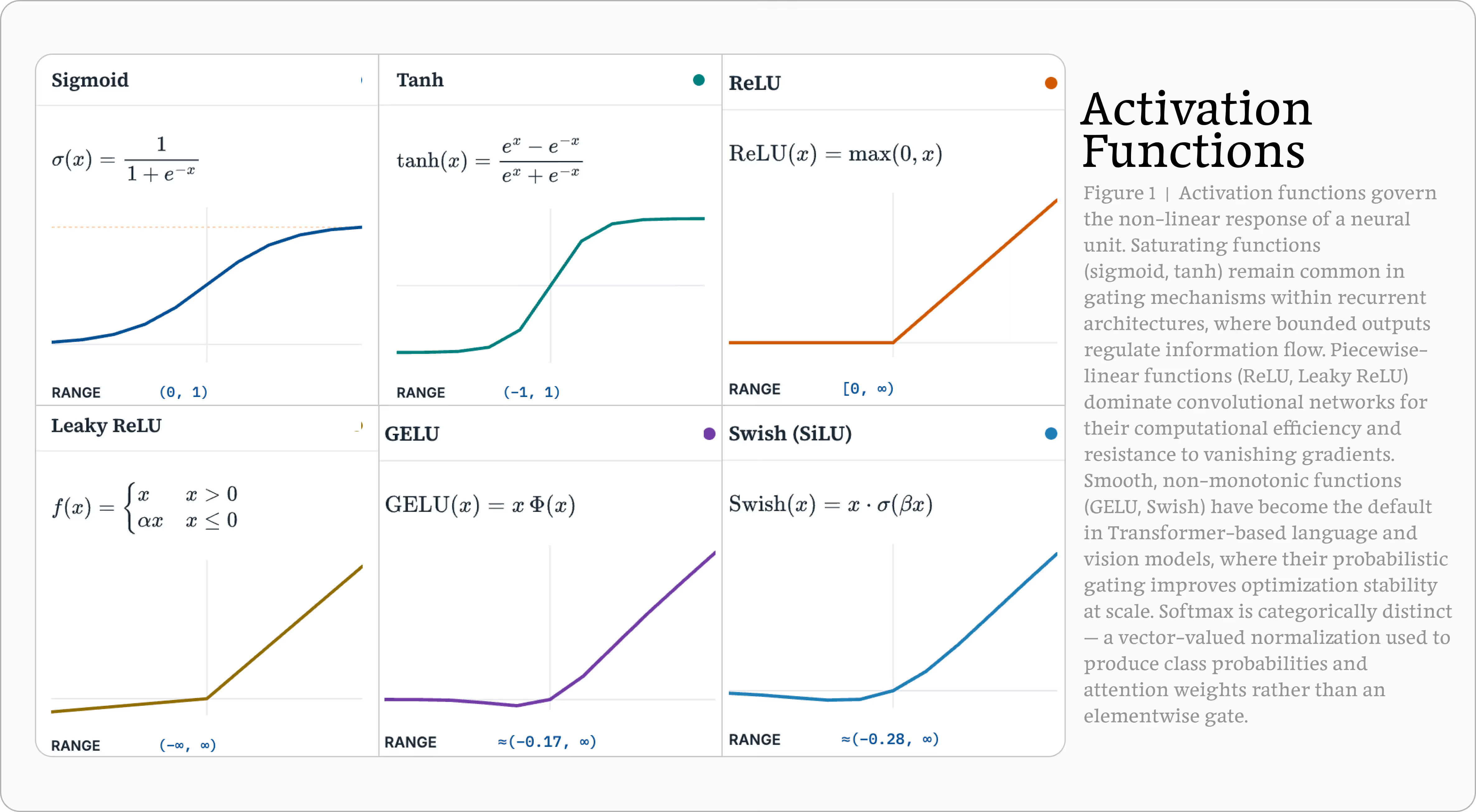
GELU and Swish
Smooth, non-monotonic activation functions increasingly used in modern architectures, particularly Transformers. GELU (Gaussian Error Linear Unit) weights the input by its value under the standard normal CDF, and Swish is defined as \( z \cdot \sigma(z) \). Both tend to slightly outperform ReLU in very deep networks, at a modest increase in computational cost.
| Function | Range | Common Use | Main Drawback |
|---|---|---|---|
| Sigmoid | (0, 1) | Binary classification output | Vanishing gradients, not zero-centered |
| Tanh | (-1, 1) | Hidden layers (older architectures), RNN gates | Vanishing gradients at saturation |
| ReLU | [0, ∞) | Hidden layers (default choice) | Dying ReLU problem |
| Leaky ReLU | (-∞, ∞) | Hidden layers, when dying ReLU is a concern | Extra hyperparameter \( \alpha \) |
| Softmax | (0, 1), sums to 1 | Multi-class classification output | Not used in hidden layers |
| GELU / Swish | (-∞, ∞) approx. | Transformers, modern deep architectures | Higher computational cost |
ReLU vs GELU: Which Should You Use?
| Aspect | ReLU | GELU |
|---|---|---|
| Shape | Hard cutoff at zero; piecewise linear | Smooth curve; small negative inputs pass through partially |
| Compute cost | Very cheap (single max operation) | More expensive (involves the Gaussian CDF or a tanh approximation) |
| Dying-neuron risk | Higher-negative inputs produce exactly zero gradient | Lower-negative inputs still carry a small, non-zero gradient |
| Typical use | CNNs, MLPs, general-purpose hidden layers | Transformers (BERT, GPT-style models), modern large-scale architectures |
| Rule of thumb | Default choice for most feedforward and convolutional networks | Preferred when training very deep Transformer stacks, where the smoothness aids optimization |
Loss Functions
A loss function (also called a cost or objective function) quantifies the gap between the network's predictions and the true target values. Training minimizes this function; the choice of loss function must match the type of task.
Mean Squared Error (MSE)
\[ \text{MSE} = \frac{1}{m} \sum_{i=1}^{m} (y^{(i)} - \hat{y}^{(i)})^2 \]The standard loss for regression tasks, where the output is a continuous numeric value. It penalizes larger errors disproportionately more due to the squaring term.
Binary Cross-Entropy
\[ \mathcal{L} = -\frac{1}{m}\sum_{i=1}^{m} \left[ y^{(i)} \log(\hat{y}^{(i)}) + (1 - y^{(i)}) \log(1 - \hat{y}^{(i)}) \right] \]Used for binary classification, typically paired with a sigmoid output activation. It measures the divergence between the true label (0 or 1) and the predicted probability.
Categorical Cross-Entropy
\[ \mathcal{L} = -\frac{1}{m}\sum_{i=1}^{m}\sum_{k=1}^{K} y_k^{(i)} \log(\hat{y}_k^{(i)}) \]The multi-class generalization of binary cross-entropy, typically paired with a softmax output layer. \( y_k^{(i)} \) is 1 for the true class and 0 otherwise (a one-hot encoding).
| Task Type | Typical Loss Function | Typical Output Activation |
|---|---|---|
| Regression | Mean Squared Error / Mean Absolute Error | Linear (none) |
| Binary classification | Binary Cross-Entropy | Sigmoid |
| Multi-class classification | Categorical Cross-Entropy | Softmax |
Forward Propagation
Forward propagation is the process of computing a network's output given an input, by passing data successively through each layer. For a network with \( L \) layers, let \( a^{[0]} = x \) be the input, and for each layer \( l = 1, \ldots, L \):
\[ z^{[l]} = W^{[l]} a^{[l-1]} + b^{[l]}, \qquad a^{[l]} = g^{[l]}(z^{[l]}) \]where \( W^{[l]} \) is the weight matrix for layer \( l \), \( b^{[l]} \) is its bias vector, \( g^{[l]} \) is its activation function, and \( a^{[l]} \) is the resulting activation output passed to the next layer. The final layer's activation \( a^{[L]} \) is the network's prediction \( \hat{y} \).
Every practical implementation performs this computation as matrix multiplication across an entire batch of examples simultaneously, rather than looping over individual inputs, which is what allows modern hardware (GPUs, TPUs) to train networks efficiently.
Worked Example
Consider a tiny network with 2 inputs, one hidden layer of 2 neurons using ReLU, and one output neuron using sigmoid. Suppose \( x = [1, 2] \), \( W^{[1]} = \begin{bmatrix} 0.5 & -0.5 \\ 0.3 & 0.8 \end{bmatrix} \), \( b^{[1]} = [0, 0] \), \( W^{[2]} = [0.6, 0.9] \), \( b^{[2]} = 0 \).
\[ z^{[1]} = \begin{bmatrix} 0.5(1) + (-0.5)(2) \\ 0.3(1) + 0.8(2) \end{bmatrix} = \begin{bmatrix} -0.5 \\ 1.9 \end{bmatrix}, \quad a^{[1]} = \text{ReLU}(z^{[1]}) = \begin{bmatrix} 0 \\ 1.9 \end{bmatrix} \] \[ z^{[2]} = 0.6(0) + 0.9(1.9) = 1.71, \quad a^{[2]} = \sigma(1.71) \approx 0.847 \]The network's prediction for this input is approximately \( 0.847 \)-if this were a binary classification problem, that would be interpreted as an 84.7% predicted probability of the positive class.
Backpropagation
Backpropagation is the algorithm that computes the gradient of the loss function with respect to every weight and bias in the network, layer by layer, working backward from the output. It is, without exaggeration, the single most important algorithm in deep learning-without an efficient way to compute these gradients, training networks with more than one or two layers would be computationally infeasible.
The Chain Rule
Backpropagation is a direct, efficient application of the calculus chain rule. For the output layer, the gradient of the loss \( \mathcal{L} \) with respect to the pre-activation \( z^{[L]} \) is:
\[ \delta^{[L]} = \frac{\partial \mathcal{L}}{\partial z^{[L]}} = \frac{\partial \mathcal{L}}{\partial a^{[L]}} \cdot g'^{[L]}(z^{[L]}) \]For every earlier layer, the error signal \( \delta^{[l]} \) is computed from the error signal of the layer after it-hence "back" propagation:
\[ \delta^{[l]} = \left( (W^{[l+1]})^{\top} \delta^{[l+1]} \right) \odot g'^{[l]}(z^{[l]}) \]where \( \odot \) denotes element-wise multiplication. Once every \( \delta^{[l]} \) is known, the gradients with respect to the weights and biases of that layer follow directly:
\[ \frac{\partial \mathcal{L}}{\partial W^{[l]}} = \delta^{[l]} (a^{[l-1]})^{\top}, \qquad \frac{\partial \mathcal{L}}{\partial b^{[l]}} = \delta^{[l]} \]Why This Matters Computationally
The key efficiency insight is that backpropagation computes gradients for all parameters in a network with \( P \) total weights in \( O(P) \) time-the same order of complexity as a single forward pass-rather than the \( O(P^2) \) or worse that would be required if gradients were estimated numerically (by perturbing each weight individually and observing the change in loss). This efficiency is precisely what makes training networks with millions or billions of parameters computationally tractable.
The Vanishing and Exploding Gradient Problems
Because \( \delta^{[l]} \) is computed by repeatedly multiplying by weight matrices and activation derivatives across many layers, two failure modes can emerge in deep networks:
- Vanishing gradients: if the relevant derivatives are consistently less than 1 (common with sigmoid/tanh), the product shrinks exponentially with depth, so early layers receive almost no learning signal.
- Exploding gradients: if the relevant values are consistently greater than 1, the product grows exponentially, causing unstable, oscillating updates or numerical overflow.
Modern practice mitigates both problems through careful weight initialization, activation functions like ReLU that do not saturate for positive inputs, gradient clipping (capping the gradient's magnitude), batch normalization, and architectural solutions such as residual (skip) connections-introduced by He et al. (2016) to train networks over 100 layers deep-and the gating mechanisms used in LSTM and GRU.
Research Perspective. Gradient pathologies remain an active research area beyond the classical vanishing/exploding framing-recent work examines phenomena such as sharp loss-landscape curvature, the interaction between learning rate and batch size at scale, and gradient behavior in very wide or very deep Transformer stacks. Skip connections and normalization layers address the symptom effectively enough for practical use, but a complete theoretical account of why deep networks train as reliably as they do is still an open problem.
Gradient Descent and Optimizers
Gradient descent is the core optimization algorithm used to update weights once backpropagation has computed gradients. The basic update rule for any parameter \( \theta \) is:
\[ \theta \leftarrow \theta - \eta \, \frac{\partial \mathcal{L}}{\partial \theta} \]where \( \eta \) is the learning rate. Because the gradient points in the direction of steepest increase of the loss, subtracting it moves the parameter toward lower loss.
Variants of Gradient Descent
- Batch gradient descent: computes the gradient using the entire training set before each update. Accurate but slow and memory-intensive for large datasets.
- Stochastic gradient descent (SGD): computes the gradient using a single example at a time. Fast per update but noisy.
- Mini-batch gradient descent: computes the gradient using a small batch (e.g., 32-256 examples) at a time. This is the practical default used in essentially all modern training, balancing speed, memory, and gradient stability.
Momentum
\[ v \leftarrow \beta v + (1 - \beta) \nabla_{\theta}\mathcal{L}, \qquad \theta \leftarrow \theta - \eta v \]Momentum accumulates a running average of past gradients, which accelerates convergence along consistent directions and dampens oscillation in directions where the gradient repeatedly changes sign.
Adam (Adaptive Moment Estimation)
Adam combines momentum with per-parameter adaptive learning rates, using running estimates of both the first moment (mean) and second moment (uncentered variance) of the gradients:
\[ m_t = \beta_1 m_{t-1} + (1-\beta_1) g_t, \qquad v_t = \beta_2 v_{t-1} + (1-\beta_2) g_t^2 \] \[ \theta \leftarrow \theta - \eta \, \frac{\hat{m}_t}{\sqrt{\hat{v}_t} + \epsilon} \]Adam is the most widely used optimizer in modern deep learning practice because it typically converges quickly and requires relatively little learning-rate tuning compared to plain SGD.
| Optimizer | Key Idea | Typical Use |
|---|---|---|
| SGD | Plain gradient step per batch | Simple baselines; sometimes generalizes better with careful tuning |
| SGD + Momentum | Accumulates velocity across steps | Computer vision training pipelines |
| RMSProp | Adaptive learning rate via squared-gradient average | RNNs, non-stationary objectives |
| Adam | Momentum + adaptive learning rates | Default choice for most modern deep learning |
Adam vs SGD: Which Should You Use?
| Aspect | SGD (with Momentum) | Adam |
|---|---|---|
| Learning rate | Single global rate, needs careful manual tuning/scheduling | Adaptive per-parameter rate, works well with less tuning |
| Convergence speed | Slower early on, especially without a tuned schedule | Typically faster, especially in early training |
| Memory overhead | Low-one velocity term per parameter | Higher-stores both first and second moment estimates per parameter |
| Generalization | Often generalizes slightly better on vision benchmarks with careful tuning | Can generalize marginally worse in some vision tasks, though the gap is often negligible |
| Typical use | Large-scale CNN training (e.g., ResNet on ImageNet) where compute budget allows tuning | Transformers, NLP, and most default deep learning workflows |
| Rule of thumb | Choose when you can afford to tune a learning-rate schedule and want the best final accuracy | Choose as a strong, low-maintenance default, especially early in a project |
Weight Initialization
How weights are initialized before training begins has a surprisingly large effect on whether a network trains successfully at all. Two naive choices both fail:
- Initializing all weights to zero: every neuron in a layer receives identical gradients and updates identically forever-a failure mode called the symmetry problem, which prevents neurons from learning different features.
- Initializing weights with excessively large random values: can immediately saturate activation functions or cause exploding gradients from the very first forward pass.
Xavier / Glorot Initialization
\[ W \sim \mathcal{U}\left(-\sqrt{\frac{6}{n_{in} + n_{out}}}, \sqrt{\frac{6}{n_{in} + n_{out}}}\right) \]Introduced by Glorot and Bengio (2010) and designed for sigmoid and tanh activations, this scheme sets the variance of initial weights based on the number of input and output connections of a layer, keeping the variance of activations and gradients roughly stable across layers.
He Initialization
\[ W \sim \mathcal{N}\left(0, \frac{2}{n_{in}}\right) \]Proposed by He et al. (2015) specifically for ReLU and its variants, which zero out roughly half of their inputs; He initialization compensates by using a larger variance than Xavier initialization would suggest. It is the standard default for modern ReLU-based networks.
Overfitting and Underfitting
These are the two fundamental failure modes of any learning system, including ANNs.
- Underfitting: the model is too simple (or undertrained) to capture the underlying pattern in the data. It performs poorly on both training and validation/test data.
- Overfitting: the model has effectively memorized the training data, including its noise and idiosyncrasies, rather than learning the general pattern. It performs very well on training data but poorly on unseen data.
| Signal | Underfitting | Overfitting |
|---|---|---|
| Training loss | High | Low |
| Validation loss | High | High (diverges from training loss) |
| Typical cause | Model too simple, too little training, excessive regularization | Model too complex relative to data size, too little regularization, too many epochs |
| Typical remedy | Increase model capacity, train longer, reduce regularization | Add regularization, gather more data, early stopping, data augmentation |
The practical goal of model development is neither of these extremes, but the sweet spot in between-often visualized as the point where validation loss is at its minimum before it starts rising again even as training loss continues to fall.
Regularization Techniques
Regularization refers to any technique that reduces overfitting by constraining a model's effective complexity or by injecting noise/redundancy that discourages memorization.
L1 and L2 Regularization (Weight Decay)
\[ \mathcal{L}_{\text{total}} = \mathcal{L} + \lambda \sum |w_i| \quad \text{(L1)}, \qquad \mathcal{L}_{\text{total}} = \mathcal{L} + \lambda \sum w_i^2 \quad \text{(L2)} \]Both add a penalty term to the loss that grows with the magnitude of the weights, discouraging the network from relying too heavily on any single connection. L1 tends to push some weights exactly to zero (producing sparsity); L2, also called weight decay, tends to shrink weights smoothly toward zero.
Dropout
Introduced by Srivastava et al. (2014), dropout randomly "turns off" a fraction of neurons (commonly 20-50%) in a layer for each training batch during training, forcing the network to not rely too heavily on any single neuron or narrow set of neurons. At inference time, all neurons are active, typically with their outputs scaled to compensate.
Early Stopping
Training is halted once validation loss stops improving for a set number of epochs (the "patience"), even if training loss is still decreasing-directly preventing the network from continuing past the point of diminishing generalization returns.
Batch Normalization
Proposed by Ioffe and Szegedy (2015), batch normalization normalizes the inputs to a layer (across a mini-batch) to have roughly zero mean and unit variance before applying a learned scale and shift. This stabilizes and often accelerates training, and provides a mild regularizing effect as a side benefit.
Data Augmentation
Artificially expands the effective size of the training set by applying label-preserving transformations to existing examples-rotating or cropping images, adding noise to audio, paraphrasing text-so the network sees more variation without requiring new labeled data.
Common Misconception. Batch normalization's original justification-reducing "internal covariate shift"-has itself been challenged by later research, which found that its main practical benefit may come from smoothing the loss landscape rather than from stabilizing layer-input distributions per se. The technique remains highly effective; it is the textbook explanation for why it works that is still debated. This is a useful reminder that an empirically successful technique can outrun a full theoretical understanding of its own mechanism.
Hyperparameters
Hyperparameters are configuration choices set before training begins, as opposed to parameters (weights and biases) that are learned during training.
| Hyperparameter | What It Controls |
|---|---|
| Learning rate | Step size of each weight update |
| Batch size | Number of examples processed before each weight update |
| Number of epochs | How many full passes over the training set are performed |
| Number of layers / neurons per layer | Model capacity and depth |
| Activation function | Non-linearity applied at each layer |
| Optimizer choice | Update rule used to adjust weights from gradients |
| Regularization strength (\( \lambda \), dropout rate) | How aggressively overfitting is penalized |
| Weight initialization scheme | Starting distribution of weights before training |
Hyperparameters are typically tuned via systematic search (grid search, random search) or more sample-efficient methods (Bayesian optimization), evaluated against a held-out validation set rather than the training or test set, to avoid biasing the final performance estimate.
Training Process: End to End
Putting every earlier section together, a typical ANN training pipeline looks like this:
- Data collection and preprocessing: gather labeled data, handle missing values, encode categorical variables, and normalize or standardize numeric features.
- Train/validation/test split: divide data (commonly 70/15/15 or 80/10/10) so that model selection and final evaluation are performed on data the model never trained on.
- Architecture selection: choose a network family (MLP, CNN, RNN, Transformer, etc.) and initial depth/width appropriate to the data type and task.
- Weight initialization: initialize weights using an appropriate scheme (He, Xavier).
- Training loop: for each epoch, iterate over mini-batches, performing forward propagation, loss computation, backpropagation, and an optimizer step for each batch.
- Validation monitoring: after each epoch, evaluate loss and relevant metrics on the validation set to track overfitting and decide when to stop.
- Hyperparameter tuning: adjust learning rate, architecture, regularization, and other hyperparameters based on validation performance, and retrain.
- Final evaluation: once satisfied, evaluate the chosen model exactly once on the held-out test set to obtain an unbiased estimate of real-world performance.
- Deployment and monitoring: deploy the trained model for inference, and continue monitoring its performance on live data, since real-world data distributions can drift over time.
Tip. Always plot training and validation loss curves together. A widening gap between them, with training loss still falling while validation loss rises, is the clearest visual signature of overfitting-and it is far more informative than looking at a single final accuracy number.
Python and PyTorch Implementation
A Neural Network from Scratch with NumPy
To make every mechanic in this article concrete, here is a complete implementation of a small feedforward network-2 inputs, one hidden layer of 4 neurons with ReLU, and a sigmoid output-with manually coded forward propagation, backpropagation, and gradient descent, trained to solve the XOR problem (which, unlike a single perceptron, a network with a hidden layer can solve):
import numpy as np

class SimpleANN:
    def __init__(self, n_input, n_hidden, n_output, lr=0.1):
        rng = np.random.default_rng(42)
        # He initialization for the ReLU hidden layer
        self.W1 = rng.normal(0, np.sqrt(2 / n_input), (n_input, n_hidden))
        self.b1 = np.zeros((1, n_hidden))
        self.W2 = rng.normal(0, np.sqrt(2 / n_hidden), (n_hidden, n_output))
        self.b2 = np.zeros((1, n_output))
        self.lr = lr

    def relu(self, z):
        return np.maximum(0, z)

    def relu_deriv(self, z):
        return (z > 0).astype(float)

    def sigmoid(self, z):
        return 1 / (1 + np.exp(-z))

    def forward(self, X):
        self.z1 = X @ self.W1 + self.b1
        self.a1 = self.relu(self.z1)
        self.z2 = self.a1 @ self.W2 + self.b2
        self.a2 = self.sigmoid(self.z2)
        return self.a2

    def backward(self, X, y):
        m = X.shape[0]
        y = y.reshape(-1, 1)

        # Output layer gradient (binary cross-entropy + sigmoid combines cleanly)
        dz2 = self.a2 - y
        dW2 = self.a1.T @ dz2 / m
        db2 = np.sum(dz2, axis=0, keepdims=True) / m

        # Hidden layer gradient (chain rule through ReLU)
        da1 = dz2 @ self.W2.T
        dz1 = da1 * self.relu_deriv(self.z1)
        dW1 = X.T @ dz1 / m
        db1 = np.sum(dz1, axis=0, keepdims=True) / m

        # Gradient descent update
        self.W2 -= self.lr * dW2
        self.b2 -= self.lr * db2
        self.W1 -= self.lr * dW1
        self.b1 -= self.lr * db1

    def compute_loss(self, y_true, y_pred):
        eps = 1e-9
        return -np.mean(y_true * np.log(y_pred + eps) +
                         (1 - y_true) * np.log(1 - y_pred + eps))

    def fit(self, X, y, epochs=5000):
        for epoch in range(epochs):
            y_pred = self.forward(X)
            loss = self.compute_loss(y.reshape(-1, 1), y_pred)
            self.backward(X, y)
            if epoch % 1000 == 0:
                print(f"Epoch {epoch}: loss = {loss:.4f}")
        return self


if __name__ == "__main__":
    # XOR dataset - not linearly separable, unsolvable by a single perceptron
    X = np.array([[0, 0], [0, 1], [1, 0], [1, 1]], dtype=float)
    y = np.array([0, 1, 1, 0], dtype=float)

    model = SimpleANN(n_input=2, n_hidden=4, n_output=1, lr=0.5)
    model.fit(X, y, epochs=5000)

    predictions = model.forward(X)
    print("Predictions:", predictions.round(3).flatten())  # ≈ [0, 1, 1, 0]
Notice this is the same forward-backward-update loop described in How ANN Works, made fully explicit in code. Unlike a single perceptron, this network solves XOR because its hidden layer can learn two separate linear boundaries and combine them non-linearly-exactly the resolution described in our perceptron article's discussion of the XOR problem.
The Same Network in PyTorch
In practice, no one hand-derives gradients for real projects-frameworks like PyTorch compute them automatically via autograd. Here is the equivalent network using PyTorch's high-level API:
import torch
import torch.nn as nn

class ANN(nn.Module):
    def __init__(self, n_input, n_hidden, n_output):
        super().__init__()
        self.fc1 = nn.Linear(n_input, n_hidden)
        self.relu = nn.ReLU()
        self.fc2 = nn.Linear(n_hidden, n_output)
        self.sigmoid = nn.Sigmoid()

    def forward(self, x):
        x = self.relu(self.fc1(x))
        x = self.sigmoid(self.fc2(x))
        return x


X = torch.tensor([[0., 0.], [0., 1.], [1., 0.], [1., 1.]])
y = torch.tensor([[0.], [1.], [1.], [0.]])

model = ANN(n_input=2, n_hidden=4, n_output=1)
criterion = nn.BCELoss()
optimizer = torch.optim.Adam(model.parameters(), lr=0.05)

for epoch in range(2000):
    optimizer.zero_grad()          # clear previous gradients
    y_pred = model(X)              # forward propagation
    loss = criterion(y_pred, y)    # compute loss
    loss.backward()                # backpropagation (autograd)
    optimizer.step()               # gradient descent update

    if epoch % 500 == 0:
        print(f"Epoch {epoch}: loss = {loss.item():.4f}")

print("Predictions:", model(X).detach().round().flatten())  # → tensor([0., 1., 1., 0.])
Every stage from the manual NumPy version maps directly onto this code: model(X) is forward propagation, criterion(y_pred, y) computes the loss, loss.backward() performs backpropagation automatically via autograd, and optimizer.step() performs the gradient descent (here, Adam) update.
A CNN Layer in a Few Lines (TensorFlow/Keras)
For contrast, here is how briefly a convolutional architecture can be expressed using high-level APIs, illustrating how the same underlying principles (weights, activations, loss, backpropagation) scale up to specialized architectures:
import tensorflow as tf
from tensorflow.keras import layers, models

model = models.Sequential([
    layers.Conv2D(32, (3, 3), activation='relu', input_shape=(28, 28, 1)),
    layers.MaxPooling2D((2, 2)),
    layers.Conv2D(64, (3, 3), activation='relu'),
    layers.MaxPooling2D((2, 2)),
    layers.Flatten(),
    layers.Dense(64, activation='relu'),
    layers.Dense(10, activation='softmax')   # 10-class classification
])

model.compile(optimizer='adam',
              loss='sparse_categorical_crossentropy',
              metrics=['accuracy'])

# model.fit(X_train, y_train, epochs=10, validation_split=0.1)
Despite the very different layer types, this is still the same fundamental training loop: forward propagation through convolutional and dense layers, a categorical cross-entropy loss, backpropagation, and Adam performing the gradient descent updates.
Real-World Applications
Artificial Neural Networks underpin a large share of software products people use every day. A representative, non-exhaustive sample:
- Computer vision: facial recognition, medical image diagnosis (e.g., detecting tumors in radiology scans), autonomous vehicle perception, quality-control defect detection in manufacturing.
- Natural language processing: machine translation, sentiment analysis, chatbots and virtual assistants, large language models for text generation and summarization.
- Speech and audio: speech-to-text transcription, voice assistants, speaker identification, music generation and recommendation.
- Finance: credit scoring, algorithmic trading signal generation, fraud detection in transaction streams.
- Healthcare: disease risk prediction from electronic health records, drug discovery via molecular property prediction, personalized treatment recommendation.
- Recommender systems: product, video, and content recommendation on e-commerce and streaming platforms.
- Robotics and control: reinforcement-learning-driven robotic manipulation and locomotion, using neural networks as function approximators for policies and value functions.
- Generative AI: image generation, text-to-image and text-to-video systems, and large-scale conversational AI assistants, virtually all built on Transformer-based ANNs.
Advantages and Disadvantages
| Advantages | Disadvantages |
|---|---|
| Can approximate highly complex, non-linear relationships | Requires large amounts of labeled data to train well, especially for deep architectures |
| Automatically learns useful features from raw data (less manual feature engineering) | Computationally expensive to train, often requiring specialized GPU/TPU hardware |
| Generalizes across many domains-vision, language, audio, tabular data | Acts largely as a "black box," making predictions difficult to interpret or explain |
| Scales well with more data and compute, often improving predictably | Prone to overfitting without careful regularization and validation |
| Backed by decades of mature tooling (PyTorch, TensorFlow) and research | Sensitive to hyperparameter choices; training can be unstable or fail to converge |
| Transfer learning allows reuse of pretrained networks across related tasks | Can inherit and amplify biases present in training data |
Common Challenges
- Data quality and quantity: ANNs are data-hungry, and poor-quality, biased, or insufficient data directly limits achievable performance regardless of architecture.
- Vanishing/exploding gradients: deep networks can struggle to propagate useful learning signal across many layers without careful initialization, normalization, and architecture design.
- Overfitting: especially likely when model capacity is large relative to available training data.
- Computational cost: training large models can require substantial time, energy, and specialized hardware, raising both financial and environmental costs.
- Interpretability: understanding why a network made a specific prediction remains an active research area (explainable AI), which matters greatly in high-stakes domains like healthcare and finance.
- Hyperparameter sensitivity: learning rate, architecture, and regularization choices can dramatically affect whether training succeeds at all.
- Distribution shift: a network trained on one data distribution can degrade significantly when deployed on data that differs systematically from its training distribution.
Best Practices
- Always establish a simple baseline (e.g., logistic regression or a small MLP) before reaching for a large, complex architecture-many problems do not require deep networks at all.
- Normalize or standardize input features; unscaled inputs can slow convergence and destabilize training.
- Use an appropriate weight initialization scheme (He for ReLU-family activations, Xavier/Glorot for sigmoid/tanh) rather than the framework's arbitrary default when it does not match your activation.
- Monitor training and validation loss together throughout training, not just a single final metric.
- Apply regularization (dropout, weight decay, early stopping) proportional to how large your model is relative to your dataset size.
- Start with Adam as a default optimizer, and use a learning-rate schedule (warmup, decay) for longer or larger training runs.
- Version and log experiments (hyperparameters, metrics, checkpoints) so results are reproducible and comparable across runs.
- Prefer an existing, well-tested architecture (ResNet, standard Transformer blocks, etc.) over a novel custom design unless you have a specific, well-understood reason to deviate.
- Evaluate on a held-out test set exactly once, at the very end, to obtain an honest estimate of real-world performance.
ANN vs Machine Learning vs Deep Learning vs Perceptron
These four terms are closely related but are not interchangeable. Understanding how they nest inside one another clears up a great deal of confusion.
24.1 ANN vs Machine Learning
Machine learning is the umbrella field of algorithms that learn patterns from data without being explicitly programmed with fixed rules-this includes linear regression, decision trees, random forests, support vector machines, and artificial neural networks. An ANN is one specific family of machine learning model, distinguished by its layered structure of interconnected neurons trained via backpropagation. Every ANN is a machine learning model; most machine learning models are not ANNs.
24.2 ANN vs Deep Learning
Deep learning refers to ANNs that have many hidden layers-"deep" architectures capable of learning hierarchical representations, where early layers learn simple features and later layers combine them into increasingly abstract concepts. A shallow ANN with a single hidden layer is still an ANN, but is not generally considered "deep learning." Every deep learning model is an ANN; not every ANN is deep enough to be called deep learning.
24.3 ANN vs Perceptron
A perceptron is a single artificial neuron using a hard step activation function, trained with the perceptron learning rule, and limited to linearly separable problems. An ANN is a network of many neuron-like units-generally using smooth, differentiable activation functions-arranged into interconnected layers and trained with backpropagation and gradient descent, capable of representing non-linear functions that a single perceptron provably cannot. See our companion article on the perceptron for a full derivation of this limitation and how stacking units resolves it.
| Term | Scope | Relationship to the Others |
|---|---|---|
| Machine Learning | Broadest-any algorithm that learns from data | Contains ANN, deep learning, and the perceptron as special cases |
| Artificial Neural Network | Layered networks of artificial neurons | A subset of machine learning; contains deep learning as a subset |
| Deep Learning | ANNs with many hidden layers | A subset of ANN, focused on depth and hierarchical representation learning |
| Perceptron | A single artificial neuron with a step activation | The historical, minimal building block that ANNs generalize and extend |
24.4 ANN vs CNN
A Convolutional Neural Network (CNN) is not a different technology from an ANN-it is an ANN with a specific connection pattern (convolutional filters with shared weights) instead of full, dense connectivity between every neuron in adjacent layers. See Section 8.3 for the full architecture.
| Aspect | Generic ANN (Fully Connected) | CNN |
|---|---|---|
| Connectivity | Every neuron connects to every neuron in the next layer | Small, shared filters slide across the input (local connectivity) |
| Parameter count | Grows quickly with input size | Much smaller due to weight sharing across spatial positions |
| Best suited for | Tabular or already-flattened feature vectors | Images and other grid-structured, spatially correlated data |
| Key property | No built-in spatial awareness | Translation invariance-detects a feature regardless of position |
24.5 ANN vs Transformer
A Transformer is likewise a specialized ANN, built primarily from self-attention layers rather than dense or convolutional layers. See Section 8.6 for the full mechanism.
| Aspect | Generic ANN (Fully Connected) | Transformer |
|---|---|---|
| Core mechanism | Fixed weighted sums between adjacent layers | Self-attention-each position dynamically weighs every other position |
| Handling of order/position | No inherent notion of sequence order | Requires explicit positional encodings to represent order |
| Parallelization | Layer-by-layer, generally straightforward to parallelize | Highly parallelizable across sequence positions, unlike RNNs |
| Best suited for | Simple, fixed-size feature vectors | Long sequences-language, code, and increasingly images and audio |
24.6 ANN vs MLP
A Multilayer Perceptron (MLP) is, in fact, the most literal, "textbook" example of an ANN: a stack of fully connected layers with non-linear activations. See Section 8.2 for details. Every MLP is an ANN; the reverse is not always true, since CNNs, RNNs, and Transformers are also ANNs but are not MLPs.
| Aspect | ANN (umbrella term) | MLP |
|---|---|---|
| Scope | Any network of artificial neurons in layers-includes MLP, CNN, RNN, Transformer | Specifically, a network of only fully connected (dense) layers |
| Typical structure | Varies by architecture family | Input layer -> one or more dense hidden layers -> output layer |
| Best suited for | Depends on the specific architecture chosen | Tabular data and simple, fixed-size feature vectors |
Interview Questions
- Derive the backpropagation update rule for a hidden layer using the chain rule.
- Why can't a network be trained with the step activation function used in the classical perceptron?
- Explain the vanishing gradient problem and describe two distinct ways to mitigate it.
- What is the Universal Approximation Theorem, and what does it not guarantee in practice?
- Compare and contrast dropout, L2 regularization, and early stopping as overfitting countermeasures.
- Why is He initialization preferred over Xavier initialization for ReLU networks?
- Explain why mini-batch gradient descent is generally preferred over both full-batch and pure stochastic gradient descent in practice.
- What structural property of CNNs makes them more parameter-efficient than fully connected networks for image data?
- How does the LSTM's gating mechanism address the shortcomings of a vanilla RNN?
- What is the fundamental architectural difference between an RNN and a Transformer, and why does it allow Transformers to parallelize training?
Frequently Asked Questions
- An Artificial Neural Network (ANN) is a computing system made of layers of interconnected artificial neurons, loosely inspired by how biological brains process information. Each connection between neurons carries a numeric weight, and the network learns by repeatedly adjusting these weights so that a given input eventually produces the desired output.
- An ANN is the general term for any network built from artificial neurons, including very shallow ones with a single hidden layer. Deep learning refers specifically to ANNs with many hidden layers-deep architectures-that learn hierarchical, increasingly abstract representations of data. Every deep learning model is an ANN, but not every ANN is deep.
- A perceptron is a single artificial neuron with a hard step activation function that can only learn linearly separable functions. An ANN is a network built from many neuron-like units-typically using smooth, differentiable activation functions-arranged across interconnected layers, which allows it to approximate complex, non-linear relationships that a lone perceptron cannot.
- An ANN learns through a repeated cycle: forward propagation pushes input data through the network to produce a prediction; a loss function measures how far that prediction is from the true label; backpropagation computes how much each individual weight contributed to that error; and an optimizer, typically some form of gradient descent, nudges every weight in the direction that reduces the error. This cycle repeats over many iterations until the network predictions are sufficiently accurate.
- The major families include Feedforward Neural Networks and Multilayer Perceptrons for general-purpose tabular problems, Convolutional Neural Networks for image and spatial data, Recurrent Neural Networks together with LSTM and GRU variants for sequential data, and Transformer-based architectures, which now dominate large-scale language and increasingly vision tasks.
- Machine learning is the broad field of algorithms that learn patterns from data, encompassing decision trees, support vector machines, random forests, and artificial neural networks among many others. An ANN is one specific family within machine learning, distinguished by its layered structure of interconnected neurons and its reliance on gradient-based training via backpropagation.
- Without a non-linear activation function, stacking any number of layers would still collapse mathematically into a single linear transformation, since a composition of linear functions is itself linear. Non-linear activation functions such as ReLU, sigmoid, and tanh are what allow a multi-layer network to approximate arbitrarily complex, non-linear functions.
- There is no universal answer-it depends on the complexity of the problem and the amount of available data. Simple tabular problems often work well with one or two hidden layers, while image recognition, language modeling, and other high-complexity tasks typically require dozens or even hundreds of layers, usually organized into specialized architectures such as CNNs or Transformers rather than a single generic stack.
Key Takeaways
- An ANN is a network of interconnected artificial neurons organized into an input layer, one or more hidden layers, and an output layer, loosely inspired by biological neurons.
- Networks learn through a repeating cycle of forward propagation, loss computation, backpropagation, and gradient-based weight updates.
- Non-linear activation functions (ReLU, sigmoid, tanh, softmax, GELU) are what give networks the ability to represent complex, non-linear relationships-without them, any depth of network collapses to a linear model.
- Different data types call for different architectures: MLPs for tabular data, CNNs for images, RNN/LSTM/GRU for sequences, and Transformers for large-scale sequence and language modeling.
- Overfitting and underfitting are the two central risks in training, managed through regularization, validation monitoring, and appropriate model capacity.
- ANN, machine learning, deep learning, and the perceptron form a nested hierarchy, not four interchangeable synonyms-precision about which term applies avoids a great deal of confusion.
The Artificial Neural Network is simultaneously simple and vast: simple in its basic unit-a weighted sum, a bias, and a non-linear activation-and vast in the range of behavior that emerges when millions or billions of such units are connected, trained, and specialized into architectures like CNNs, RNNs, and Transformers. Every concept in this guide, from a single neuron's forward pass to the self-attention mechanism inside a modern language model, is a variation on the same core idea introduced by the perceptron and made trainable at scale by backpropagation.
The most productive way to use this material is not to memorize it, but to build with it: implement a small network from scratch, watch it fail to converge until the learning rate or initialization is fixed, watch it overfit until regularization is added, and watch its behavior change as you swap one architecture for another. That hands-on cycle-predict, measure error, adjust, repeat-is, fittingly, exactly the same loop the network itself uses to learn.