Perceptron Explained: The Origin of Neural Networks
Abstract
This article traces the Perceptron from its biological and historical roots to its complete mathematical formulation, learning algorithm, and provable limitations. It covers the McCulloch-Pitts neuron, the geometry of linear decision boundaries, a full derivation and proof sketch of the Perceptron Convergence Theorem, worked numerical examples, from-scratch Python and PyTorch implementations, and a rigorous treatment of the XOR problem-closing with the historical and mathematical motivation for Multi-Layer Perceptrons.
Why the Perceptron Matters
Every modern deep learning system-every Transformer, every convolutional network, every large language model-is built from a single repeating computational unit: a weighted sum of inputs, a bias, and a nonlinearity. That unit is the perceptron. Understanding it is not a historical curiosity; it is the atomic building block from which everything else in deep learning is composed.
The perceptron is also one of the rare ideas in computer science whose success, near-death, and resurrection form a complete arc. It was invented with grand ambitions, proven to have a fundamental limitation, and then rehabilitated as the seed from which multi-layer networks-and eventually the entire deep learning revolution-grew. This article walks through that full arc: where the idea came from, exactly how it works mathematically, how it learns, why it provably fails on certain problems, and how that very failure motivated the next major architecture.
By the end of this article you will be able to derive the perceptron's decision rule from first principles, implement its learning algorithm from scratch in Python and PyTorch, prove mathematically why it cannot solve XOR, and understand precisely why this limitation motivated the Multi-Layer Perceptron.
Historical Motivation and Earlier Computational Models
Before the perceptron, computation was understood almost entirely through the lens of symbolic logic and fixed circuits. Alan Turing's abstract machine (1936) established what was computable in principle, but said nothing about how a physical or biological system might learn to compute a function from examples. Early digital computers of the 1940s executed rigid, hand-programmed instructions-they could not adapt their own behavior based on data.
The central unanswered question of the era was this: could a machine learn its own rules, rather than being told them explicitly? Researchers working at the intersection of neuroscience, logic, and engineering began to ask whether the brain's biological machinery offered a template. If neurons in the brain could somehow implement logical functions, perhaps an artificial system built the same way could learn from experience rather than from a programmer's instructions.
This question motivated two major developments that directly preceded the perceptron:
- McCulloch and Pitts's formal neuron (1943): a mathematical model showing that networks of simple threshold units could, in principle, compute any logical proposition.
- Hebbian learning theory (1949): psychologist Donald Hebb proposed that the biological basis of learning is the strengthening of connections between neurons that fire together-often summarized as "cells that fire together, wire together."
Frank Rosenblatt, working at the Cornell Aeronautical Laboratory, synthesized these two ideas in 1958 into a concrete, trainable computational model: the perceptron. Unlike the static McCulloch-Pitts neuron, whose weights had to be set by hand, the perceptron came with an algorithm for learning those weights automatically from labeled examples. This was the crucial innovation-not just a model of a neuron, but a model of how a neuron could learn.
Biological Inspiration: From Neurons to Nodes
A biological neuron receives electrochemical signals through its dendrites, integrates them in the cell body (soma), and-if the combined signal exceeds a threshold-fires an electrical pulse down its axon to other neurons. This all-or-nothing firing behavior is the single most important abstraction borrowed by artificial neurons: a neuron sums its inputs and produces an output only if that sum is large enough.
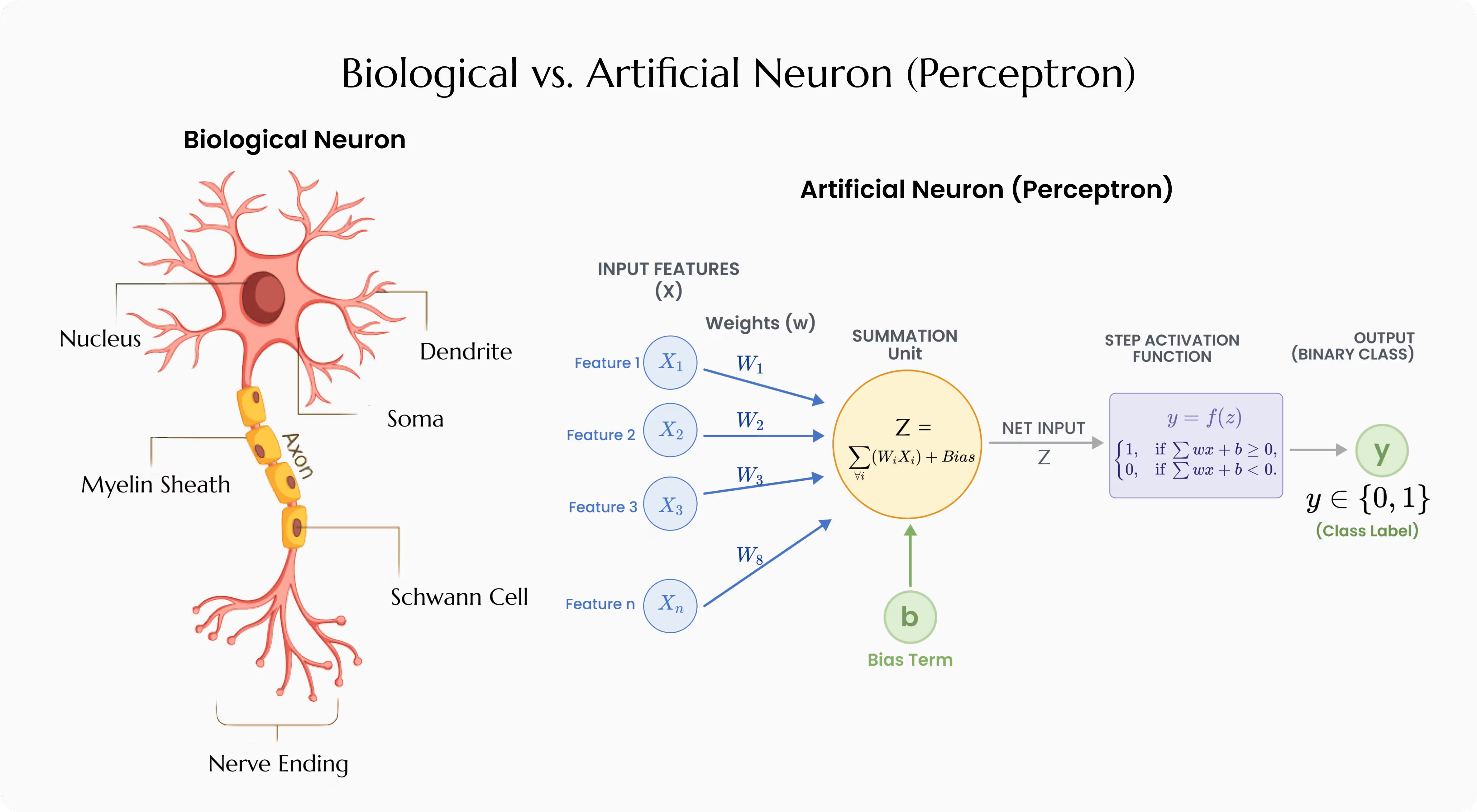
The analogy is deliberately loose. Real neurons are vastly more complex-they exhibit temporal dynamics, stochastic firing, thousands of synapses with varying plasticity, and chemical modulation that has no direct analogue in the perceptron's clean algebra. The artificial neuron keeps only the abstraction that mattered for computation: weighted inputs, an integration step, and a thresholded output. This simplification is precisely what made the model mathematically tractable while still being a source of genuine algorithmic insight.
| Biological Component | Artificial Analogue | Function |
|---|---|---|
| Dendrites | Inputs \( x_1, \ldots, x_n \) | Receive incoming signals |
| Synaptic strength | Weights \( w_1, \ldots, w_n \) | Scale the importance of each input |
| Resting potential / threshold | Bias \( b \) | Shifts the firing threshold |
| Soma (cell body) | Weighted summation \( \sum w_i x_i + b \) | Integrates all incoming signals |
| Axon firing / not firing | Step activation function | Produces a binary output decision |
The McCulloch-Pitts Neuron
The McCulloch-Pitts (MP) neuron published in 1943 ↗ is the direct mathematical ancestor of the perceptron. It is a binary threshold unit: given binary inputs \( x_1, x_2, \ldots, x_n \in \{0, 1\} \), it computes
\[ y = \begin{cases} 1 & \text{if } \sum_{i=1}^{n} x_i \geq \theta \\ 0 & \text{otherwise} \end{cases} \]where \( \theta \) is a fixed threshold. Crucially, the MP neuron has no weights-every input contributes equally-and no learning mechanism whatsoever. Its threshold and connectivity had to be designed by hand to compute a specific logical function (AND, OR, NOT), much like designing a logic-gate circuit.
McCulloch and Pitts proved something remarkable for their time: networks of these simple units, connected appropriately, could compute any logical proposition expressible in propositional logic. This was a landmark theoretical result establishing that networks of simple threshold units are computationally universal in a logical sense. But it left open the practical question that mattered most for building intelligent systems: how would the correct threshold and connectivity ever be discovered automatically, from data, rather than hand-engineered?
The perceptron answers exactly that question. Rosenblatt's key generalization was to introduce real-valued, learnable weights \( w_i \) for each input, replacing the MP neuron's implicit equal weighting, and to pair this with an algorithm that adjusts those weights automatically based on classification errors. This single change-from fixed, hand-set connections to learned, real-valued weights-is what transforms a static logical model into a genuine learning machine.
Perceptron Architecture and Mathematical Formulation
5.1 Inputs, Weights, and Bias
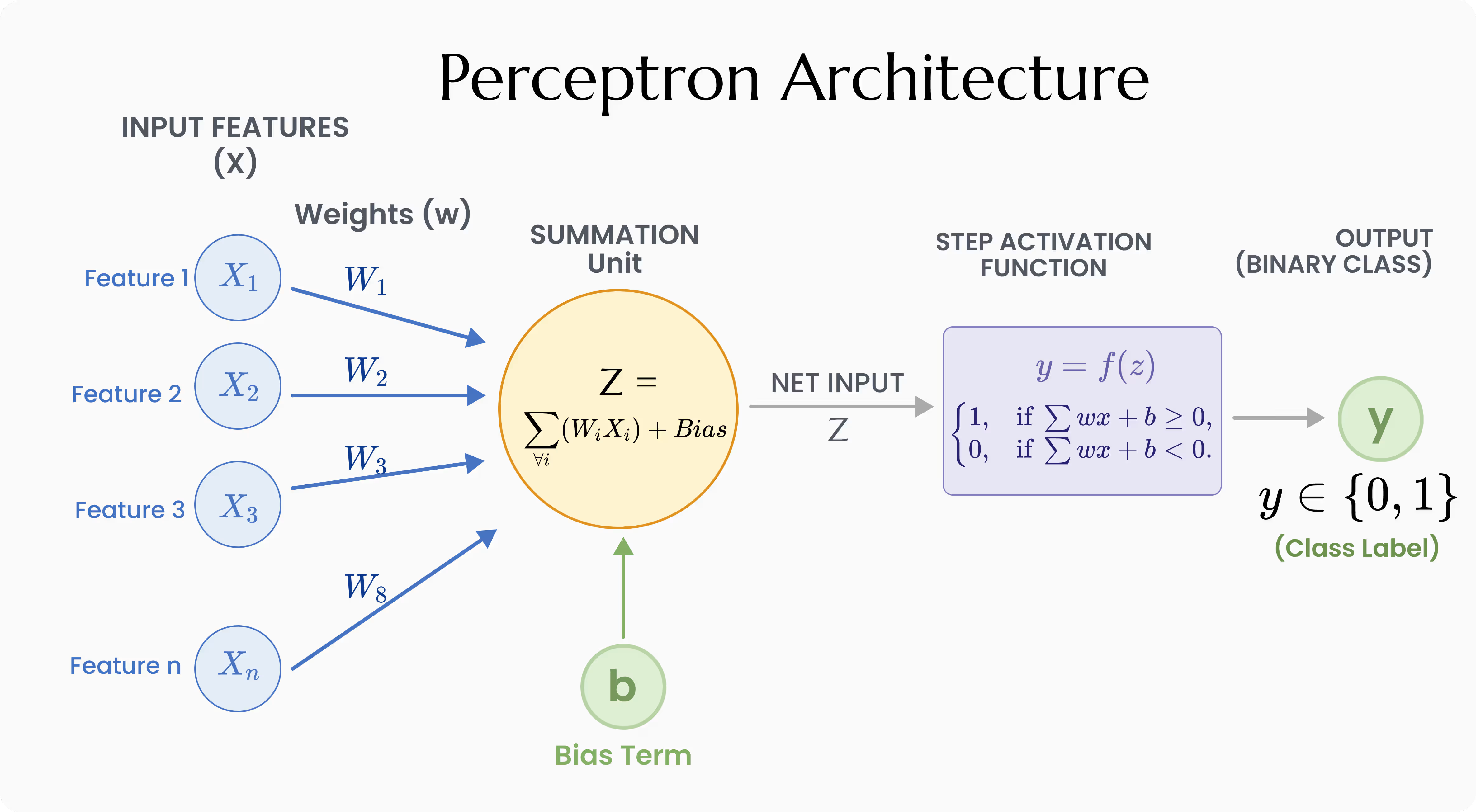
A perceptron receives an input vector \( \mathbf{x} = (x_1, x_2, \ldots, x_n) \in \mathbb{R}^n \), where each \( x_i \) is a numeric feature. Each input is associated with a learnable real-valued weight \( w_i \in \mathbb{R} \), representing how strongly that feature influences the output. There is additionally a single bias term \( b \in \mathbb{R} \) (sometimes written as a weight \( w_0 \) attached to a constant input \( x_0 = 1 \)), which allows the decision boundary to be shifted away from the origin.
5.2 Weighted Summation
The perceptron first computes a weighted sum of its inputs, called the net input or pre-activation:
\[ z = \sum_{i=1}^{n} w_i x_i + b = \mathbf{w}^{\top} \mathbf{x} + b \]Geometrically, \( z \) measures the signed distance (scaled by \( \|\mathbf{w}\| \)) of the point \( \mathbf{x} \) from a hyperplane defined by \( \mathbf{w} \) and \( b \). This single linear expression is the entire "computation" performed before the activation function is applied.
5.3 The Step Activation Function
The net input \( z \) is passed through a nonlinear activation function to produce the final binary output. The classical perceptron uses the Heaviside step function:
\[ \hat{y} = f(z) = \begin{cases} 1 & \text{if } z \geq 0 \\ 0 & \text{if } z < 0 \end{cases} \]Some formulations use \( \{-1, +1\} \) labels instead of \( \{0, 1\} \), in which case the step function becomes the sign function, \( f(z) = \text{sign}(z) \). Both conventions are mathematically equivalent; this article uses \( \{0, 1\} \) unless otherwise noted.
Putting it all together, the complete perceptron function is:
\[ \boxed{\hat{y} = f\left(\sum_{i=1}^{n} w_i x_i + b\right)} \]
5.4 Vector and Matrix Formulation
For a single example, using the augmented-weight trick (folding the bias into the weight vector by appending a constant \( 1 \) to the input), we can write:
\[ \tilde{\mathbf{w}} = \begin{bmatrix} b \\ w_1 \\ \vdots \\ w_n \end{bmatrix}, \quad \tilde{\mathbf{x}} = \begin{bmatrix} 1 \\ x_1 \\ \vdots \\ x_n \end{bmatrix}, \quad \hat{y} = f(\tilde{\mathbf{w}}^{\top} \tilde{\mathbf{x}}) \]For a full dataset of \( m \) examples stacked as rows of a matrix \( \mathbf{X} \in \mathbb{R}^{m \times n} \), predictions for the entire dataset can be computed in one matrix operation:
\[ \hat{\mathbf{y}} = f(\mathbf{X}\mathbf{w} + b) \]where \( f \) is applied element-wise. This vectorized form is what every practical implementation (NumPy, PyTorch, TensorFlow) uses instead of looping over examples one at a time.
Decision Boundaries and Geometric Intuition
The equation \( \mathbf{w}^{\top}\mathbf{x} + b = 0 \) defines a hyperplane in \( \mathbb{R}^n \)-a line when \( n = 2 \), a plane when \( n = 3 \), and a general hyperplane for higher dimensions. This hyperplane is the perceptron's decision boundary: every point on one side is classified as 1, and every point on the other side is classified as 0.
The weight vector \( \mathbf{w} \) is orthogonal to this hyperplane and points in the direction of increasing \( z \)-that is, toward the region classified as 1. The bias \( b \) controls how far the hyperplane is shifted from the origin along that direction. This geometric picture explains, in a single image, both what a perceptron can and cannot do: it can only ever carve space with one straight cut.
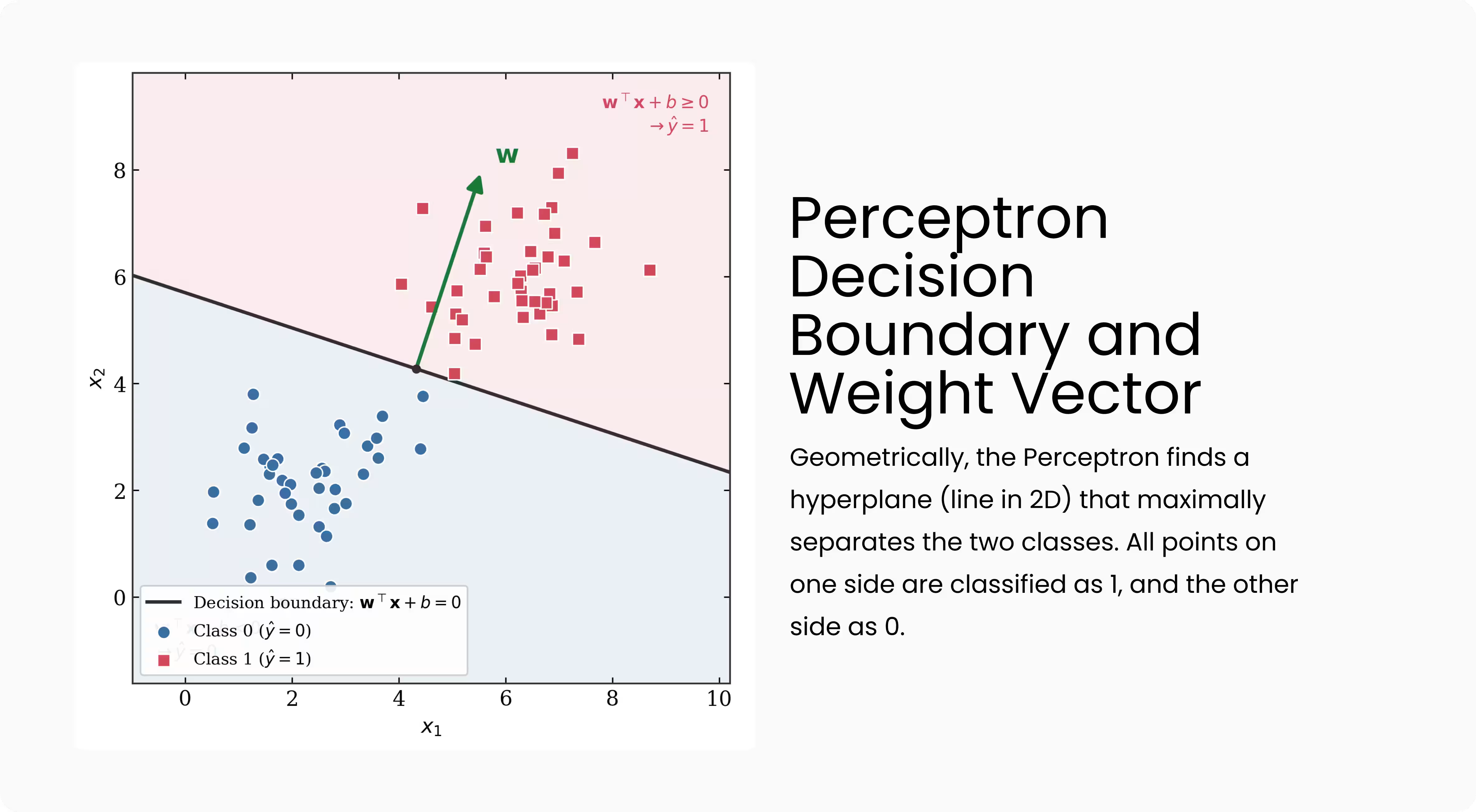
This leads directly to the single most important structural property of the perceptron: it is a linear classifier. It can correctly classify a dataset if and only if that dataset is linearly separable-meaning there exists at least one hyperplane that perfectly separates the two classes. If no such hyperplane exists, no choice of weights, no amount of training time, and no learning rate will ever produce a perfect perceptron classifier for that data. This constraint will become the crux of the XOR problem discussed later in this article.
The Perceptron Learning Algorithm
Intuition
The learning algorithm's rule is disarmingly simple: if the prediction is correct, do nothing; if it is wrong, nudge the weights in the direction that would have made it more correct. This is an error-driven update-unlike gradient descent on a smooth loss, the perceptron rule is derived directly from the misclassification itself, not from differentiating a loss function (which is impossible here, since the step function is not differentiable).
The Update Rule
For a training example \( (\mathbf{x}, y) \) with true label \( y \) and predicted label \( \hat{y} \), the weights and bias are updated as:
\[ \mathbf{w} \leftarrow \mathbf{w} + \eta (y - \hat{y}) \, \mathbf{x} \] \[ b \leftarrow b + \eta (y - \hat{y}) \]where \( \eta > 0 \) is the learning rate. Notice the term \( (y - \hat{y}) \): if the prediction is correct, \( y - \hat{y} = 0 \) and no update occurs. If the true label is 1 but the perceptron predicted 0, \( (y - \hat{y}) = 1 \), and the weights are nudged in the direction of \( \mathbf{x} \), increasing \( z \) for similar future inputs. If the true label is 0 but the perceptron predicted 1, weights are nudged in the opposite direction.
Full Training Algorithm
- Initialize weights \( \mathbf{w} \) and bias \( b \) to zero or small random values.
- For each training example \( (\mathbf{x}^{(i)}, y^{(i)}) \) in the dataset:
- Compute \( z = \mathbf{w}^{\top}\mathbf{x}^{(i)} + b \) and \( \hat{y} = f(z) \).
- Update: \( \mathbf{w} \leftarrow \mathbf{w} + \eta(y^{(i)} - \hat{y})\mathbf{x}^{(i)} \), \( b \leftarrow b + \eta(y^{(i)} - \hat{y}) \).
- Repeat step 2 for multiple epochs until no example is misclassified, or a maximum number of epochs is reached.
This procedure is called online or stochastic learning because weights are updated after every single example rather than after processing the whole dataset at once.
The Perceptron Convergence Theorem
Statement
The Perceptron Convergence Theorem, proved by Rosenblatt and later formalized rigorously by Novikoff (1962), states:
If a training dataset is linearly separable with margin \( \gamma > 0 \), the perceptron learning algorithm will find a separating hyperplane in a finite number of weight updates, bounded by \( (R/\gamma)^2 \), where \( R \) is the radius of the smallest ball containing all training points.
Proof Sketch
Assume there exists an optimal weight vector \( \mathbf{w}^{*} \) (with \( \|\mathbf{w}^{*}\| = 1 \) for normalization) that separates the data with margin \( \gamma \), meaning \( y^{(i)} (\mathbf{w}^{*\top} \mathbf{x}^{(i)}) \geq \gamma \) for every example. The proof proceeds by tracking two quantities across updates: the projection of the current weight vector \( \mathbf{w}_k \) onto \( \mathbf{w}^{*} \), and the squared norm \( \|\mathbf{w}_k\|^2 \).
Every time a mistake is made and an update occurs, one can show two facts. First, the dot product \( \mathbf{w}_k \cdot \mathbf{w}^{*} \) increases by at least \( \gamma \) with each mistake, since the update moves the weight vector in the direction consistent with the true label. Second, the squared norm \( \|\mathbf{w}_k\|^2 \) increases by at most \( R^2 \) with each mistake, because the input vectors are bounded by \( R \). Combining a lower bound on the dot product's growth with an upper bound on the norm's growth (and using the Cauchy-Schwarz inequality, since \( \mathbf{w}_k \cdot \mathbf{w}^{*} \leq \|\mathbf{w}_k\| \|\mathbf{w}^{*}\| \)) yields an upper bound on the total number of mistakes \( k \):
\[ k \leq \left(\frac{R}{\gamma}\right)^2 \]The key insight is intuitive even without the full algebra: every mistake makes measurable, bounded progress toward alignment with a separating solution. Since progress is bounded below per step and the total possible "distance" to travel is finite, the number of mistakes must be finite-hence the algorithm terminates.
What Happens When Data Is Not Linearly Separable
The theorem's converse is equally important: if no separating hyperplane exists, the bound \( (R/\gamma)^2 \) is undefined (there is no \( \gamma > 0 \)), and the algorithm provably does not converge-it will continue making updates indefinitely, cycling through weight configurations without ever reaching zero misclassifications. This is exactly the situation that arises with XOR, discussed in Section 13.
Worked Numerical Example
Consider learning the logical AND function, which is linearly separable. The training set is:
| \( x_1 \) | \( x_2 \) | \( y \) (AND) |
|---|---|---|
| 0 | 0 | 0 |
| 0 | 1 | 0 |
| 1 | 0 | 0 |
| 1 | 1 | 1 |
Initialize \( w_1 = 0, w_2 = 0, b = 0 \), with learning rate \( \eta = 1 \). We process examples in order.
Example (0, 0), y = 0: \( z = 0(0) + 0(0) + 0 = 0 \), so \( \hat{y} = f(0) = 1 \) (since \( z \geq 0 \)). This is wrong (\( y = 0 \)). Update: \( w_1 \leftarrow 0 + 1(0-1)(0) = 0 \), \( w_2 \leftarrow 0 + 1(0-1)(0) = 0 \), \( b \leftarrow 0 + 1(0-1) = -1 \).
Example (0, 1), y = 0: \( z = 0(0) + 0(1) - 1 = -1 \), so \( \hat{y} = f(-1) = 0 \). This is correct-no update.
Example (1, 0), y = 0: \( z = 0(1) + 0(0) - 1 = -1 \), so \( \hat{y} = 0 \). Correct-no update.
Example (1, 1), y = 1: \( z = 0(1) + 0(1) - 1 = -1 \), so \( \hat{y} = f(-1) = 0 \). This is wrong (\( y = 1 \)). Update: \( w_1 \leftarrow 0 + 1(1-0)(1) = 1 \), \( w_2 \leftarrow 0 + 1(1-0)(1) = 1 \), \( b \leftarrow -1 + 1(1-0) = 0 \).
After one full epoch, weights are \( w_1 = 1, w_2 = 1, b = 0 \). Running a second epoch through all four examples with these weights correctly classifies (0,0)→0, (0,1)→0 (\(z=1\), which is actually misclassified-let's verify: \(z = 1(0)+1(1)+0 = 1 \geq 0 \to \hat y = 1\), wrong again). This shows perceptron training typically requires several epochs of adjustment before convergence; continuing this process for a few more epochs converges to a stable separating solution such as \( w_1 = 1, w_2 = 1, b = -1 \), under which:
\[ z_{(0,0)} = -1 \to 0, \quad z_{(0,1)} = 0 \to 1 \text{ (boundary case)}, \quad z_{(1,0)} = 0 \to 1 \text{ (boundary case)}, \quad z_{(1,1)} = 1 \to 1 \]A cleaner converged solution that strictly separates all four points is \( w_1 = 1, w_2 = 1, b = -1.5 \), giving \( z_{(0,0)} = -1.5, z_{(0,1)} = -0.5, z_{(1,0)} = -0.5, z_{(1,1)} = 0.5 \)-correctly producing \( \hat y = 0 \) for the first three and \( \hat y = 1 \) only for (1,1), exactly matching AND. This illustrates the full learning loop end to end: initialize, predict, compare, update, and repeat until convergence.
Python and PyTorch Implementation from Scratch
Pure Python / NumPy Implementation
The perceptron learning algorithm maps almost line-for-line onto code. Here is a complete, minimal implementation using only NumPy:
import numpy as np

class Perceptron:
    def __init__(self, n_inputs, learning_rate=1.0, n_epochs=20):
        self.w = np.zeros(n_inputs)
        self.b = 0.0
        self.lr = learning_rate
        self.n_epochs = n_epochs

    def step(self, z):
        return np.where(z >= 0, 1, 0)

    def predict(self, X):
        z = X @ self.w + self.b
        return self.step(z)

    def fit(self, X, y):
        for epoch in range(self.n_epochs):
            errors = 0
            for xi, yi in zip(X, y):
                z = np.dot(self.w, xi) + self.b
                y_hat = self.step(z)
                update = self.lr * (yi - y_hat)
                self.w += update * xi
                self.b += update
                errors += int(update != 0.0)
            if errors == 0:
                print(f"Converged after {epoch + 1} epochs")
                break
        return self


if __name__ == "__main__":
    # AND gate dataset
    X = np.array([[0, 0], [0, 1], [1, 0], [1, 1]])
    y = np.array([0, 0, 0, 1])

    model = Perceptron(n_inputs=2, learning_rate=1.0, n_epochs=20)
    model.fit(X, y)

    print("Weights:", model.w, "Bias:", model.b)
    print("Predictions:", model.predict(X))   # → [0 0 0 1]
This implementation mirrors the algorithm from Section 7 exactly: predict, compare, update, repeat. Notice that errors == 0 is the convergence check-once a full epoch produces zero updates, the algorithm has found a separating hyperplane and stops early.
10.2 PyTorch Implementation
While PyTorch is designed around gradient-based learning, we can implement the true perceptron rule (not gradient descent) using a linear layer purely as a container for weights and bias, and apply the manual update rule ourselves:
import torch

class PerceptronTorch:
    def __init__(self, n_inputs, learning_rate=1.0, n_epochs=20):
        self.w = torch.zeros(n_inputs)
        self.b = torch.zeros(1)
        self.lr = learning_rate
        self.n_epochs = n_epochs

    def step_fn(self, z):
        return (z >= 0).float()

    def predict(self, X):
        z = X @ self.w + self.b
        return self.step_fn(z)

    def fit(self, X, y):
        for epoch in range(self.n_epochs):
            errors = 0
            for i in range(X.shape[0]):
                xi, yi = X[i], y[i]
                z = torch.dot(self.w, xi) + self.b
                y_hat = self.step_fn(z)
                update = self.lr * (yi - y_hat)
                self.w += update * xi
                self.b += update
                errors += int(update.abs().item() > 0)
            if errors == 0:
                print(f"Converged after {epoch + 1} epochs")
                break
        return self


if __name__ == "__main__":
    X = torch.tensor([[0., 0.], [0., 1.], [1., 0.], [1., 1.]])
    y = torch.tensor([0., 0., 0., 1.])

    model = PerceptronTorch(n_inputs=2)
    model.fit(X, y)
    print("Weights:", model.w, "Bias:", model.b)
    print("Predictions:", model.predict(X))   # → tensor([0., 0., 0., 1.])
Note that this deliberately avoids torch.autograd and loss.backward()-because the step function has zero gradient almost everywhere, standard backpropagation cannot train it. This non-differentiability is precisely why later networks replaced the step function with smooth activations like sigmoid, tanh, and ReLU, enabling gradient-based training via backpropagation.
Computational Complexity
| Operation | Time Complexity | Space Complexity |
|---|---|---|
| Single forward pass (prediction) | \( O(n) \) | \( O(n) \) |
| Single weight update | \( O(n) \) | \( O(n) \) |
| One full epoch (m examples) | \( O(mn) \) | \( O(n) \) |
| Full training (k epochs, linearly separable) | \( O(kmn) \), bounded by \( O\left(\left(\frac{R}{\gamma}\right)^2 n\right) \) mistakes | \( O(n) \) |
Here \( n \) is the number of input features, \( m \) is the number of training examples, and \( k \) is the number of epochs. Each individual update is extremely cheap-just a scalar multiply-add over the weight vector-which is why the perceptron was computationally practical even on the limited hardware of the late 1950s.
Advantages and Limitations
| Advantages | Limitations |
|---|---|
| Extremely simple to implement and understand | Can only solve linearly separable problems |
| Guaranteed convergence in finite steps if data is linearly separable | Does not converge at all if data is not linearly separable |
| Computationally cheap-\( O(n) \) per update | Step activation is non-differentiable; incompatible with gradient descent |
| Online learning-updates one example at a time | Cannot model non-linear relationships (e.g., XOR) |
| Forms the conceptual and mathematical basis for all later neural networks | No probabilistic output (hard 0/1 decision only, no confidence score) |
The XOR Problem and Why Single-Layer Perceptrons Fail
The XOR Function
The exclusive-OR (XOR) function is defined as:
| \( x_1 \) | \( x_2 \) | XOR |
|---|---|---|
| 0 | 0 | 0 |
| 0 | 1 | 1 |
| 1 | 0 | 1 |
| 1 | 1 | 0 |
Mathematical Proof of Non-Separability
Suppose, for contradiction, that a perceptron with weights \( w_1, w_2 \) and bias \( b \) correctly computes XOR. Then the following four inequalities must all hold simultaneously (using \( \hat y = 1 \iff z \geq 0 \)):
\[ \begin{aligned} (0,0) \to 0: &\quad b < 0 \\ (0,1) \to 1: &\quad w_2 + b \geq 0 \\ (1,0) \to 1: &\quad w_1 + b \geq 0 \\ (1,1) \to 0: &\quad w_1 + w_2 + b < 0 \end{aligned} \]Adding the second and third inequalities gives \( w_1 + w_2 + 2b \geq 0 \), which implies \( w_1 + w_2 \geq -2b \). But the fourth inequality states \( w_1 + w_2 < -b \). Combining these:
\[ -2b \leq w_1 + w_2 < -b \quad \Longrightarrow \quad -2b < -b \quad \Longrightarrow \quad -b < 0 \quad \Longrightarrow \quad b > 0 \]This directly contradicts the first inequality, which required \( b < 0 \). Since assuming a solution exists leads to a logical contradiction, no values of \( w_1, w_2, b \) can satisfy all four constraints simultaneously. This is a formal proof, not an empirical observation: XOR is provably unrepresentable by a single-layer perceptron, for any weights whatsoever.
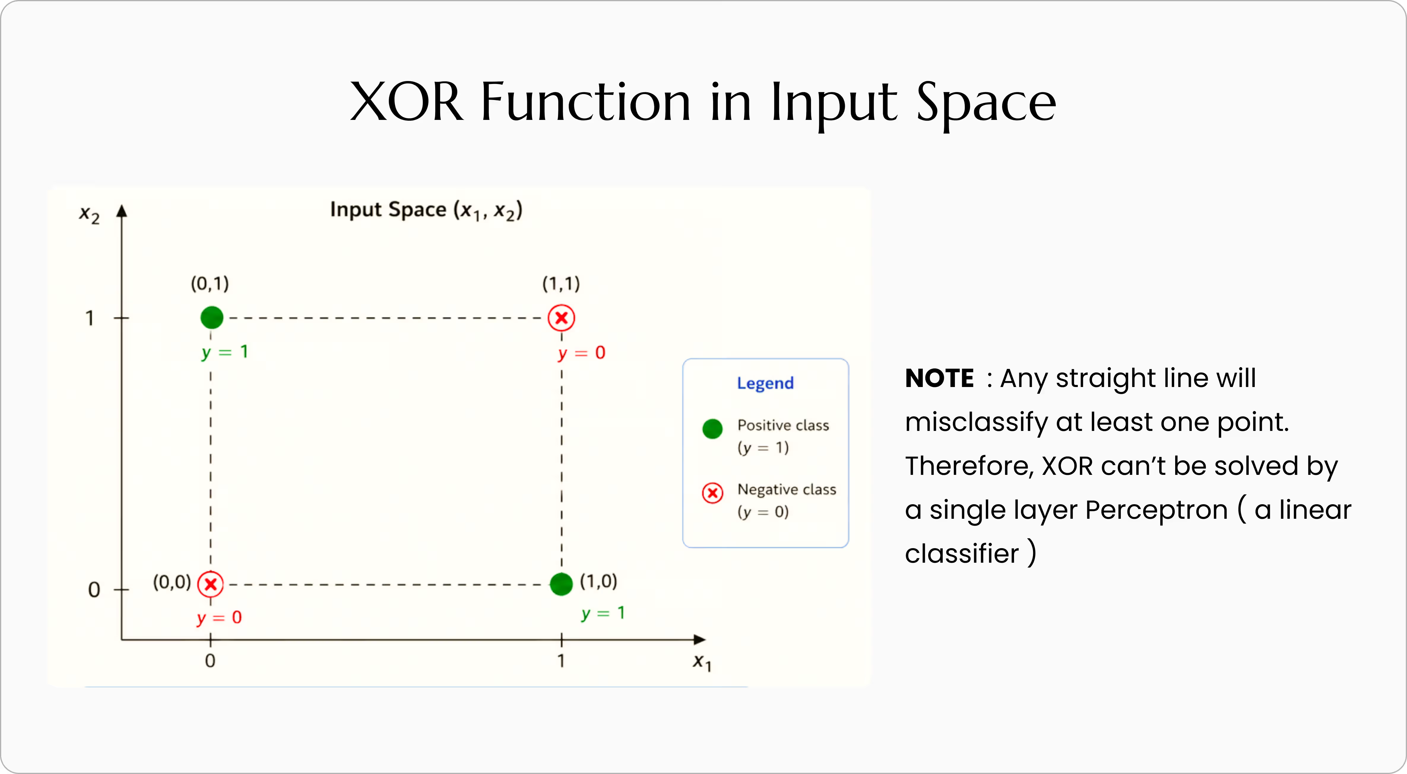
The Geometric Reason
Geometrically, XOR's positive examples, (0,1) and (1,0), sit on opposite corners of the unit square from its negative examples, (0,0) and (1,1). Any single straight line that separates one diagonal pair from the other would have to simultaneously curve around both-something a straight line, by definition, cannot do. XOR requires two lines (or one non-linear boundary), which is fundamentally beyond what a single linear decision boundary can express.
Historical Impact: Minsky and Papert
Marvin Minsky and Seymour Papert's 1969 book Perceptrons formalized this and related limitations rigorously, proving that single-layer perceptrons cannot compute any function that is not linearly separable. Their analysis was mathematically sound and specific to single-layer networks, but its chilling effect on the field was broader: funding and enthusiasm for neural network research declined sharply through the 1970s, a period now referred to as part of the first AI winter. It would take over a decade, and the rediscovery of backpropagation for training multi-layer networks, before neural networks regained mainstream credibility.
How This Limitation Motivated the Multi-Layer Perceptron
The proof in Section 13 is not merely a curiosity about one toy function-it is a statement about the entire class of functions a single linear decision boundary can represent. Many practically important problems, including XOR, are not linearly separable, so a fundamentally more expressive architecture was required.
The resolution turns out to be conceptually simple: stack perceptron-like units in layers, so that the output of one layer becomes the input to the next. A hidden layer of two perceptron-like units can each learn one of the two lines needed to carve up XOR's input space, and a final output unit can combine their results-effectively learning a non-linear decision boundary out of several linear pieces. This composition of simple linear units, stacked and interconnected, is the seed idea behind the Multi-Layer Perceptron (MLP)
Realizing this idea in practice required two further breakthroughs that this article does not detail here: replacing the non-differentiable step function with a smooth activation function, and discovering an efficient way to compute weight updates across many stacked layers-the backpropagation algorithm. Together, these transform the single perceptron's linear boundary into the universal function approximators that underlie all of modern deep learning. The Multi-Layer Perceptron, and the mathematics that makes it trainable, is the natural next topic once the perceptron itself is fully understood.
Perceptron at a Glance
| Property | Single-Layer Perceptron | Multi-Layer Perceptron (preview) |
|---|---|---|
| Decision boundary | One linear hyperplane | Piecewise non-linear (composed of many hyperplanes) |
| Activation function | Step function (non-differentiable) | Smooth functions (sigmoid, tanh, ReLU) |
| Training method | Perceptron learning rule | Gradient descent + backpropagation |
| Can solve XOR? | No (provably) | Yes |
| Convergence guarantee | Guaranteed only if linearly separable | No global guarantee, but empirically effective |
Common Misconceptions
- "A perceptron is the same as a modern neural network neuron." Not quite-a perceptron specifically uses a hard step activation and the perceptron learning rule. A modern neuron shares the weighted-sum-plus-bias structure but uses smooth activations trained via gradient descent.
- "The perceptron learning algorithm is a form of gradient descent." It is not. The step function has zero gradient almost everywhere, so the update rule is derived directly from the sign of the classification error, not from differentiating a loss function.
- "More training will eventually let a perceptron solve XOR." No amount of training helps. The limitation is a mathematical impossibility proven in Section 13, not a matter of insufficient optimization.
- "Minsky and Papert proved neural networks can't work." They proved a narrower, precise result about single-layer perceptrons and linear separability. Multi-layer networks were not covered by their impossibility proof and were already known conceptually, though practical training methods came later.
- "The bias term is optional." Without a bias, the decision boundary is forced to pass through the origin, which severely limits which linearly separable problems can be solved at all.
Best Practices When Working With Perceptrons
- Always check whether your data is linearly separable before relying on a single-layer perceptron; if not, use a Multi-Layer Perceptron instead.
- Normalize or standardize input features-perceptron convergence speed depends on the geometry (radius \( R \)) of the input space.
- Set a maximum epoch limit even on separable data, as a safety net against slow convergence with small margins \( \gamma \).
- Use the perceptron as a pedagogical and diagnostic tool: if it fails to converge, that is itself useful evidence that your data may not be linearly separable.
- For any real-world classification task, prefer a differentiable model (logistic regression, MLP) trained with gradient descent, since it will also provide probabilistic confidence estimates.
Interview Questions
- Derive the perceptron learning rule and explain the role of each term.
- State and explain the Perceptron Convergence Theorem. What happens if the data is not linearly separable?
- Prove mathematically why a single-layer perceptron cannot represent the XOR function.
- Why can't the perceptron be trained using standard backpropagation?
- What is the geometric interpretation of the weight vector and bias in a perceptron?
- How does the McCulloch-Pitts neuron differ from Rosenblatt's perceptron?
- What role does the learning rate \( \eta \) play in convergence speed and stability?
- How would you modify a perceptron to output a probability instead of a hard 0/1 decision?
- Explain how stacking perceptron-like units into layers resolves the XOR limitation.
- What is the computational complexity of one perceptron training epoch, and why?
Exercises
- Implement the perceptron learning algorithm from scratch and train it on the OR function. Verify it converges and report the final weights.
- Using the proof technique from Section 13.2, show algebraically why the NAND function can be represented by a single perceptron while XOR cannot.
- Modify the Python implementation to record and plot the number of misclassifications per epoch. Observe how this count reaches zero for linearly separable data but oscillates for XOR.
- Prove that the decision boundary of a perceptron is invariant to positive scalar multiplication of \( (\mathbf{w}, b) \)-that is, \( (\mathbf{w}, b) \) and \( (c\mathbf{w}, cb) \) for \( c > 0 \) define the same classifier.
- Given a dataset with margin \( \gamma = 0.1 \) and radius \( R = 5 \), compute the theoretical upper bound on the number of mistakes guaranteed by the Perceptron Convergence Theorem.
Frequently Asked Questions
- A perceptron is the simplest artificial neuron: it takes several numeric inputs, multiplies each by a learned weight, adds a bias, and passes the result through a step function to produce a binary output (0 or 1). It functions as a linear binary classifier that separates two classes with a straight line, plane, or hyperplane.
- No. A single-layer perceptron can only learn linearly separable functions. XOR is not linearly separable-no single straight line can correctly separate its positive and negative examples-so a perceptron cannot represent it regardless of how long it is trained or what weights are tried.
- Frank Rosenblatt introduced the perceptron in 1958 at the Cornell Aeronautical Laboratory, building on the earlier McCulloch-Pitts neuron model from 1943 and Donald Hebb's theories of synaptic learning.
- The single-layer perceptron itself is rarely deployed directly in modern applications because of its linear limitations, but it remains foundational: it is the conceptual building block of every neuron in modern deep neural networks, including Multi-Layer Perceptrons, convolutional networks, and beyond.
- A classical perceptron uses a hard step activation function and the perceptron learning rule. A modern artificial neuron has the same weighted-sum-plus-bias structure but typically uses a differentiable activation function (sigmoid, tanh, ReLU) and is trained with gradient descent and backpropagation, which the discontinuous step function does not support.
- It converges in a finite number of steps if and only if the training data is linearly separable. This is guaranteed by the Perceptron Convergence Theorem. If the data is not linearly separable, the algorithm will oscillate indefinitely and never converge.
- The perceptron learning rule updates weights only when a prediction is wrong: w ← w + η(y - ŷ)x, where η is the learning rate, y is the true label, ŷ is the predicted label, and x is the input vector. Correct predictions produce no update.
- Minsky and Papert's 1969 book Perceptrons mathematically proved that single-layer perceptrons cannot represent XOR or other non-linearly-separable functions. This result was widely (and somewhat unfairly) interpreted as a fundamental limitation of neural networks in general, contributing to a decline in funding and interest known as the first AI winter.
The perceptron is deceptively simple: a weighted sum, a bias, and a threshold. Yet within that simplicity lies the origin of an entire field. It formalized the idea that a machine could learn its own decision rule from labeled examples rather than being programmed with one, and it came with a mathematically guaranteed learning procedure-the first of its kind.
Its limitation is just as important as its capability. The proof that a single-layer perceptron cannot represent XOR is not a footnote; it is the precise mathematical boundary that separates what linear models can do from what non-linear ones can. Understanding that boundary-and why stacking simple units into layers pushes past it-is the conceptual bridge from the perceptron to the Multi-Layer Perceptron, and from there, to every modern deep learning architecture built on the same foundational unit.