Exponential Distribution

What Is an Exponential Distribution?

In probability theory and statistics, the Exponential distribution is the continuous probability distribution that describes the amount of time (or distance, or any other continuous quantity) that passes before a single event occurs, given that events happen independently and at a known constant average rate \( \lambda \) (lambda). It is the standard model for waiting times: how long until the next customer walks into a shop, how long a light bulb keeps working before it fails, how long until the next earthquake, or how many kilometers a car travels before its next breakdown. See the formula below for the precise mathematical definition.

The Exponential distribution is inseparable from the Poisson distribution: if the number of events occurring in a fixed interval of time follows a Poisson distribution with rate \( \lambda \), then the gap between any two consecutive events follows an Exponential distribution with that same rate \( \lambda \) (see the Poisson process connection). The two distributions are two views of one process — Poisson counts how many events happen, Exponential measures how long until the next one. This makes the Exponential distribution the natural continuous counterpart of the discrete Geometric distribution, and both share a rare and defining trait covered in detail below: the memoryless property.

The Formula

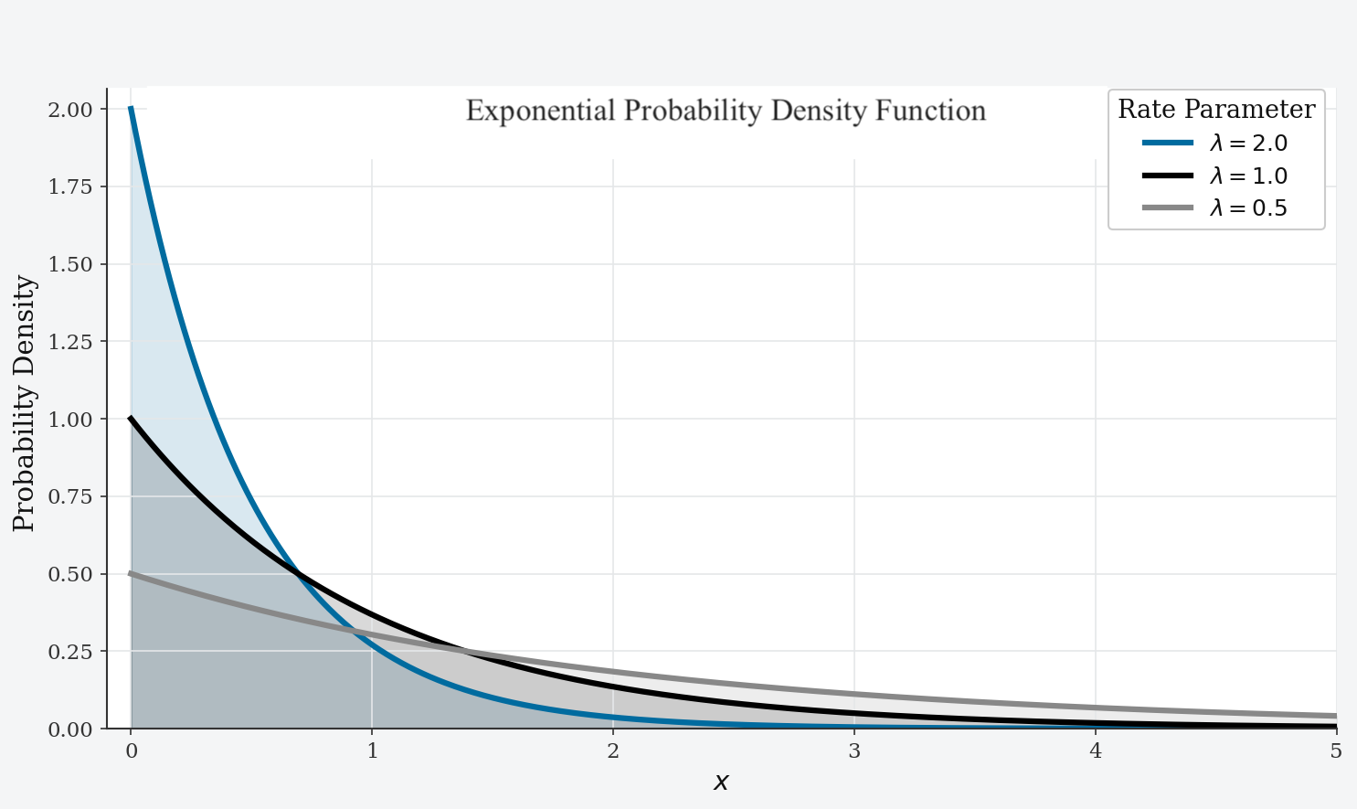
The probability density function (PDF) of an Exponential distribution, which gives the relative likelihood of the waiting time landing near a particular value \( x \), is:

and \( f(x) = 0 \) for any \( x < 0 \), since negative waiting times are not possible. Here \( \lambda > 0 \) is the rate parameter — the average number of events per unit time — and \( e \approx 2.71828 \) is Euler's number. Unlike the normal distribution's two-parameter bell curve, a single number \( \lambda \) fully determines the entire shape and position of the Exponential density (see Notation & Parameters for the constraint it must satisfy).

The curve starts at its maximum height, \( f(0) = \lambda \), and decays continuously and monotonically toward zero as \( x \) grows — there is no rise, no peak elsewhere, and no symmetry: short waiting times are always the most likely outcome, and the probability of a very long wait shrinks exponentially rather than tapering gently. As with any valid PDF, the total area under the curve integrates to exactly \( 1 \), which follows directly from the fact that \( \int_0^{\infty} \lambda e^{-\lambda x}\,dx = \left[-e^{-\lambda x}\right]_0^{\infty} = 1 \).

Notation & Parameters

An Exponential distribution with rate \( \lambda \) is written compactly as:

read as "\( X \) is exponentially distributed with rate \( \lambda \)." Several conventions and constraints apply:

• \( \lambda > 0 \) must be strictly positive — a rate of zero would mean events never happen at all, which is not a valid Exponential distribution.
• Some sources parameterize the distribution by its scale, \( \beta = 1/\lambda \) (the mean waiting time), writing the density as \( f(x) = \frac{1}{\beta} e^{-x/\beta} \) instead. Both parameterizations describe the same family of curves; the convention in use should always be confirmed before values are substituted, since mixing them up inverts every calculation.
• The support of the distribution — the set of values \( X \) can take — is all non-negative real numbers, \( x \in [0, \infty) \). This reflects that the quantity being modeled is almost always a duration, a distance, or another inherently non-negative measurement.
• \( \lambda \) carries units of "events per unit time" (or per unit distance, and so on), while the mean waiting time \( 1/\lambda \) carries the reciprocal units — time per event. Keeping these straight matters in applied problems: a rate of \( \lambda = 4 \) calls per hour implies a mean waiting time of \( 1/4 \) hour, or 15 minutes, between calls.

Core Properties

Beyond the formula and its single parameter, the Exponential distribution has a set of defining mathematical properties that explain both its shape and its widespread use as a waiting-time model.

Strictly Decreasing Density

Unlike the bell-shaped normal distribution, the Exponential density has no interior peak to speak of: its single highest point is at the boundary \( x = 0 \), and it falls off monotonically from there. There is no symmetry between short and long waits — the distribution is always right-skewed, reflecting that a wait of zero (or near zero) is the single most likely outcome, however small \( \lambda \) is.

Mean, Median, and Mode Diverge

Because the curve is neither symmetric nor peaked away from zero, its three principal measures of central tendency separate from one another, in contrast to the normal distribution, where they always coincide:

• the mode (the most probable value) sits at \( x = 0 \), the boundary of the support,
• the median is \( \dfrac{\ln 2}{\lambda} \approx \dfrac{0.693}{\lambda} \), and
• the mean is \( \dfrac{1}{\lambda} \), always strictly larger than the median (see Moments for the derivation).

The gap between mean and median is a direct consequence of the distribution's long right tail: a handful of unusually long waits pull the average upward, even though the great majority of individual waits fall below it.

Variance and Standard Deviation

The variance, \( \operatorname{Var}(X) = 1/\lambda^2 \), measures the average squared distance of waiting times from the mean. Its square root, the standard deviation \( \sigma = 1/\lambda \), turns out to be numerically identical to the mean itself — a distinctive signature: for an Exponential variable, the typical spread of outcomes is always exactly as large as the average outcome.

Skewness

Skewness measures the asymmetry of a distribution. Regardless of the value chosen for \( \lambda \), the Exponential distribution always has:

This constant, strongly positive skewness reflects the same long right tail described above, and it does not change shape with \( \lambda \) — only the scale of the curve changes (see Shape as \( \lambda \) Varies).

Kurtosis

Kurtosis describes how heavy or light a distribution's tails are relative to its peak. The Exponential distribution has a kurtosis of:

The strongly positive excess kurtosis marks the Exponential distribution as leptokurtic: its tail carries meaningfully more probability than a normal distribution with matching variance would, consistent with the fact that unusually long waits, while individually rare, are not negligible.

Scale Family

The Exponential distribution is a scale family: if \( X \sim \operatorname{Exp}(\lambda) \), then \( cX \sim \operatorname{Exp}(\lambda/c) \) for any constant \( c > 0 \). Rescaling the units in which time is measured — switching from minutes to hours, say — leaves the distribution exponential, only with a correspondingly rescaled rate.

The Memoryless Property

The single most distinctive fact about the Exponential distribution is that it is memoryless: the probability of waiting some additional amount of time for the next event does not depend at all on how long has already been waited. Formally, for any \( s, t \geq 0 \):

In words: if a light bulb has already survived \( s \) hours without failing, the probability it survives at least \( t \) more hours is exactly the same as the probability a brand-new bulb survives \( t \) hours. The bulb, in a precise mathematical sense, does not "remember" that it has already been running — its remaining lifetime is statistically identical to its original lifetime, as if the clock had just been reset.

This is a genuinely unusual property, and a striking theorem in probability theory establishes that the Exponential distribution is the only continuous probability distribution with support on \( [0, \infty) \) that has it. Every other continuous waiting-time distribution — the Weibull or gamma distributions among them — incorporates some notion of aging, whether components wear out and become more likely to fail over time, or "warm up" and become less likely to fail the longer they have already run. Only the Exponential distribution treats every instant as a fresh start.

The derivation follows directly from the survival function \( P(X > x) = e^{-\lambda x} \):

which uses only the algebraic fact that exponentials of sums split into products, \( e^{-\lambda(s+t)} = e^{-\lambda s} \cdot e^{-\lambda t} \). The geometric distribution is the discrete analogue: it is the unique memoryless distribution on the non-negative integers, for exactly the same algebraic reason applied to a discrete rather than continuous sum.

Shape as \( \lambda \) Varies

The rate parameter \( \lambda \) controls both the height and the steepness of the density simultaneously, since \( f(0) = \lambda \) is the curve's starting height and also the coefficient controlling how fast it decays.

• Large \( \lambda \) (a high event rate) produces a tall curve that starts high and plunges toward zero almost immediately — events happen fast, so long waits are extremely unlikely.
• Small \( \lambda \) (a low event rate) produces a short, gently sloping curve that stretches out over a much wider range of \( x \) — events happen slowly, so long waits remain reasonably plausible far out along the x-axis.

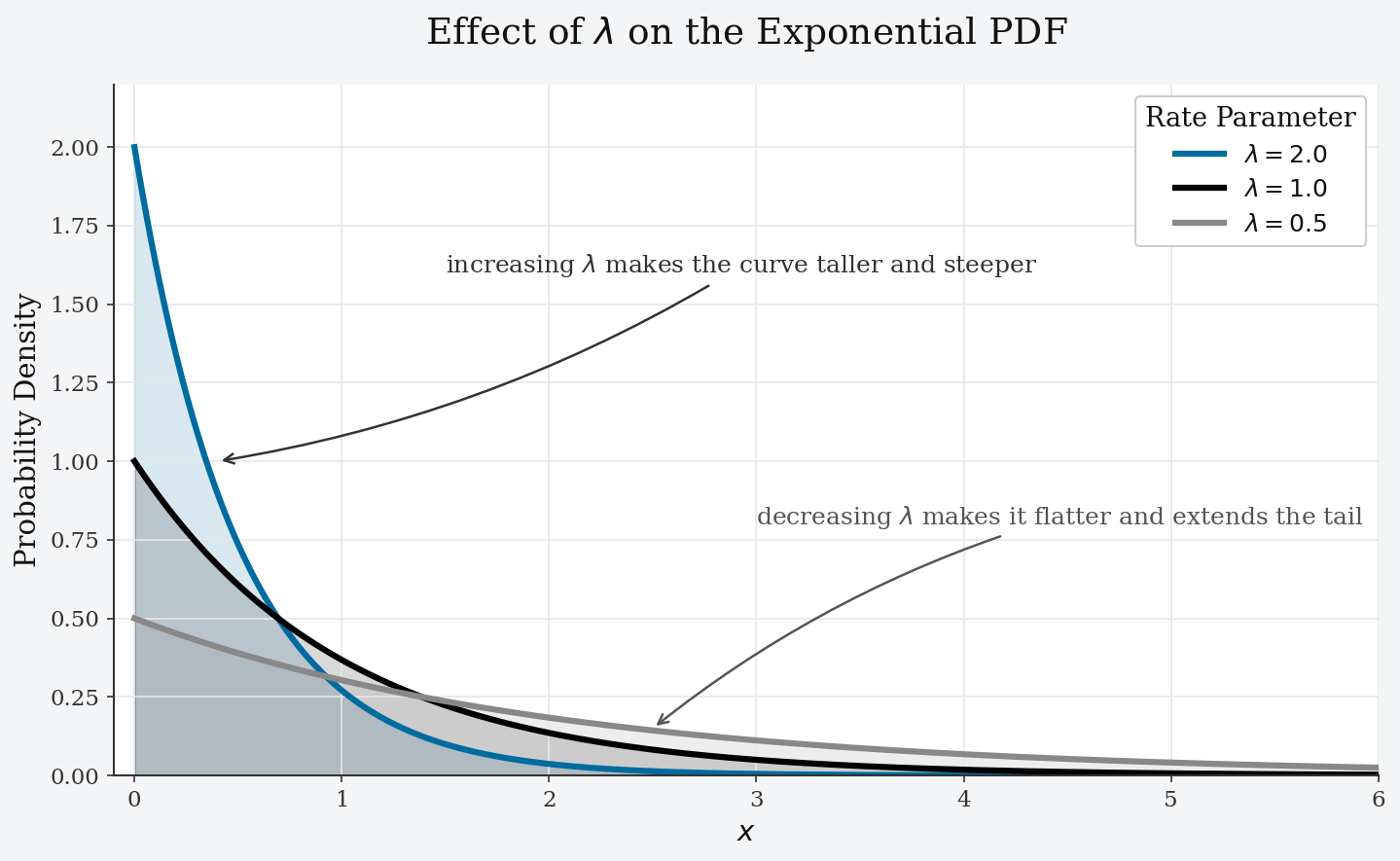
Because \( \lambda \) is the only free parameter, every Exponential curve is a rescaled version of every other — the underlying shape (monotonically decreasing, skewness of exactly \( 2 \), and so on) never changes; only the horizontal and vertical scale does.

Moments & Generating Functions

The mean (expected value) of an Exponential random variable is:

This is the intuitive result: if events happen at rate \( \lambda \) per unit time, the average wait between them is the reciprocal, \( 1/\lambda \) units of time.

The variance follows from \( \operatorname{Var}(X) = E[X^2] - (E[X])^2 \), where \( E[X^2] = 2/\lambda^2 \):

The moment generating function (MGF), which compactly encodes every moment of the distribution, is:

The restriction \( t < \lambda \) is essential: for \( t \geq \lambda \), the defining integral \( \int_0^{\infty} e^{tx}\lambda e^{-\lambda x}\,dx \) diverges, since the growth of \( e^{tx} \) would overwhelm the decay of \( e^{-\lambda x} \). Differentiating \( M_X(t) \) once and evaluating at \( t = 0 \) recovers the mean \( 1/\lambda \); differentiating twice recovers \( E[X^2] = 2/\lambda^2 \), matching the variance derived directly above.

The k-th raw moment has a clean closed form for every positive integer \( k \):

which reduces to the mean when \( k=1 \) and to \( E[X^2] \) when \( k=2 \), and generalizes the pattern to any higher moment needed.

Cumulative Distribution Function

The cumulative distribution function (CDF) gives the probability that the waiting time is at most \( x \):

and \( F(x) = 0 \) for \( x < 0 \). Unlike the normal distribution's CDF, which has no elementary closed form and must be evaluated via lookup tables or numerical approximation, the Exponential CDF is a single, exactly computable expression — one of the practical conveniences that makes the distribution easy to work with by hand.

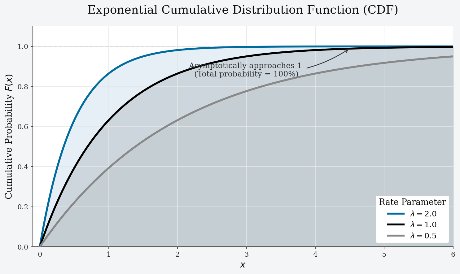
The CDF is used directly to compute interval probabilities: \( P(a \leq X \leq b) = F(b) - F(a) = e^{-\lambda a} - e^{-\lambda b} \) for any \( 0 \leq a \leq b \). It is also the basis for the standard method of generating Exponential random numbers via inversion (see Generating Exponential Random Numbers).

Survival & Hazard Functions

Two functions closely related to the CDF are especially prominent in reliability engineering and survival analysis, fields where the Exponential distribution is a foundational model.

Survival Function

The survival function \( S(x) \), also written \( \bar{F}(x) \), gives the probability that the event has not yet happened by time \( x \) — equivalently, the probability a component is still functioning after \( x \) units of time:

This is precisely the expression used in the derivation of the memoryless property above.

Hazard Function

The hazard function (or failure rate) \( h(x) \) gives the instantaneous rate of failure at time \( x \), conditional on having survived that long:

The hazard function is constant, equal to \( \lambda \) at every instant, regardless of how long the component has already survived. This constant-hazard property is exactly the memoryless property restated in reliability language: components modeled as Exponential neither wear out nor improve with age, which makes the Exponential distribution a natural (if simplified) model for the "useful life" middle segment of the classic bathtub curve of failure rates, flanked by early "infant mortality" failures and later wear-out failures that require distributions such as the Weibull instead.

Worked Example

Suppose customer support tickets arrive at a help desk at an average rate of \( \lambda = 3 \) tickets per hour, and the arrivals are well modeled as a Poisson process (independent arrivals at a constant average rate). The waiting time \( X \), in hours, until the next ticket arrives follows \( X \sim \operatorname{Exp}(3) \).

1. What is the expected waiting time until the next ticket?

2. What is the probability the next ticket arrives within 10 minutes (\( x = 1/6 \) hour)?

There is roughly a 39.4% chance the next ticket arrives within the next 10 minutes.

3. Given that 15 minutes (\( 0.25 \) hour) have already passed with no ticket, what is the probability of waiting at least 10 more minutes?

By the memoryless property, this is identical to the probability of a fresh wait of at least 10 minutes, regardless of the 15 minutes already elapsed:

The answer, about 60.7%, would be exactly the same whether the desk had already been waiting 0 minutes, 15 minutes, or 3 hours — a direct illustration of why the memoryless property makes hand calculation with the Exponential distribution unusually convenient.

Estimating \( \lambda \) from Data

Given a sample of \( n \) independent waiting times \( x_1, x_2, \ldots, x_n \) drawn from an Exponential distribution, the maximum likelihood estimator of the rate parameter is:

the reciprocal of the sample mean waiting time. This falls out directly from maximizing the log-likelihood \( \ell(\lambda) = n\ln\lambda - \lambda\sum x_i \) with respect to \( \lambda \), and it matches the intuitive method-of-moments estimate obtained by simply setting the theoretical mean \( 1/\lambda \) equal to the observed sample mean \( \bar{x} \) and solving. In the customer-support example above, observing an average gap of, say, 18 minutes (\( 0.3 \) hour) across many tickets would yield an estimate of \( \hat{\lambda} = 1/0.3 \approx 3.33 \) tickets per hour.

The estimator \( \hat{\lambda} \) is slightly biased for finite \( n \), and an unbiased alternative, \( \tilde{\lambda} = \frac{n-1}{\sum x_i} \), is sometimes used instead when the sample size is small; the two estimates converge as \( n \) grows large.

The Poisson Process Connection

The relationship between the Exponential and Poisson distributions is not a coincidence of formula but a mathematical identity: both describe the exact same Poisson process — a sequence of events occurring independently and at a constant average rate \( \lambda \) — viewed through two different lenses.

• Fix a time interval and count the events inside it: that count follows a Poisson\( (\lambda t) \) distribution, where \( t \) is the interval's length.
• Fix a starting point and measure the gap until the next event: that gap follows an Exponential\( (\lambda) \) distribution.

The two can be derived from one another directly. The event "the next arrival takes longer than \( x \)" is logically identical to the event "zero arrivals occur in the interval \( [0, x] \)." Setting the Poisson probability of zero events, \( P(N=0) = \frac{(\lambda x)^0 e^{-\lambda x}}{0!} = e^{-\lambda x} \), equal to the Exponential survival function \( P(X > x) = e^{-\lambda x} \) shows the two expressions are one and the same — the identity used earlier in Survival & Hazard Functions.

This connection also explains the memoryless property intuitively: because a Poisson process has no memory of past arrivals by construction (each interval's count is independent of every other), the wait until the next arrival, viewed from any starting instant, looks statistically identical — whether that instant is the very start of the process or fifteen minutes after the last arrival.

Related Distributions

• Poisson distribution — the discrete count of events in a fixed interval of the same process for which the Exponential distribution gives the continuous gap between events (see above).
• Gamma distribution — the sum of \( k \) independent \( \operatorname{Exp}(\lambda) \) variables follows a Gamma\( (k, \lambda) \) distribution; when \( k \) is a positive integer this special case is called the Erlang distribution, historically developed to model the total waiting time across \( k \) successive phone-call arrivals.
• Geometric distribution — the discrete analogue of the Exponential distribution, counting trials rather than measuring continuous time until the first success; both are the unique memoryless distributions in their respective (discrete and continuous) settings.
• Weibull distribution — a generalization that adds a shape parameter, allowing the hazard function to increase or decrease with time instead of remaining constant; the Exponential distribution is the special case where the Weibull shape parameter equals \( 1 \).
• Minimum of Exponentials — if \( X_1, \ldots, X_n \) are independent with rates \( \lambda_1, \ldots, \lambda_n \), then \( \min(X_1,\ldots,X_n) \) is itself Exponential, with rate \( \lambda_1 + \cdots + \lambda_n \) — the basis for modeling "whichever of several independent failure modes happens first."
• Laplace distribution — sometimes called the "double exponential" distribution, formed by reflecting the Exponential density about zero to produce a symmetric, two-tailed distribution.
• Uniform distribution — connected via the standard inversion method: applying \( -\ln(U)/\lambda \) to a \( \operatorname{Uniform}(0,1) \) draw \( U \) produces an Exponential\( (\lambda) \) draw (see Generating Exponential Random Numbers).

Generating Exponential Random Numbers

Because the Exponential CDF has a simple closed-form inverse, generating Exponential random numbers is one of the most direct applications of the inverse transform sampling method.

Starting from a draw \( U \sim \operatorname{Uniform}(0,1) \), setting \( U = F(x) = 1-e^{-\lambda x} \) and solving for \( x \) gives:

and, since \( U \) and \( 1-U \) share the same \( \operatorname{Uniform}(0,1) \) distribution, the simpler equivalent form \( X = -\ln(U)/\lambda \) is used in practice. Each uniform draw maps to exactly one Exponential draw, with no rejection or iteration required — a contrast with distributions like the normal distribution, whose inverse CDF has no elementary closed form and requires methods such as Box–Muller or the Ziggurat algorithm instead.

In practice, this transform is rarely implemented by hand: libraries such as NumPy (numpy.random.exponential(scale)) or SciPy's scipy.stats.expon.rvs(scale) handle the conversion internally — using \( \text{scale} = 1/\lambda \), the mean waiting time, rather than \( \lambda \) directly, a convention worth double-checking before passing arguments.

A Short History

The Exponential distribution's mathematical roots trace back to the same 17th-century work on radioactive decay and continuous-time processes that gave rise to the underlying differential equation \( dN/dt = -\lambda N \), whose solution \( N(t) = N_0 e^{-\lambda t} \) is the exponential decay law from which the distribution takes its name. As a formal probability distribution in its own right, it emerged alongside the development of the Poisson process in the early 20th century, once the mathematics of counting rare independent events (see the history of the Poisson distribution) was extended to the continuous gaps between those events.

A pivotal figure in this development was the Danish engineer Agner Krarup Erlang, who between 1909 and the early 1920s built the foundations of queueing theory while working for the Copenhagen Telephone Company. Erlang modeled the time between successive telephone calls as Exponential, and the total waiting time across several calls using what is now called the Erlang distribution (see Related Distributions) — work that remains the theoretical backbone of telecommunications and call-center capacity planning today.

Through the mid-20th century, the distribution's memoryless property was formalized and proven unique to it among continuous distributions, cementing its role as the default starting point for reliability engineering and survival analysis, fields that matured rapidly after the Second World War alongside growing industrial and biomedical demand for models of component and patient lifetimes.

Where It Shows Up

Any scenario reducible to "how long until the next independent, constant-rate event happens" is, in principle, Exponential. A selection of concrete examples across engineering, statistics, and machine learning:

• Reliability engineering — time-to-failure for electronic components during their constant-hazard "useful life" phase is the textbook Exponential application, central to mean time between failures (MTBF) calculations.
• Queueing theory — the time between customer arrivals or the service time per customer in classic queueing models (such as the M/M/1 queue) is modeled as Exponential, building directly on Erlang's original telephony work.
• Survival analysis — patient survival time after a diagnosis or treatment is sometimes modeled with an Exponential baseline hazard, particularly as a simplifying assumption before moving to more flexible models such as the Weibull or Cox proportional-hazards frameworks.
• Radioactive decay — the time until a given radioactive atom decays follows an Exponential distribution, the continuous counterpart to the discrete count of decays used to define a substance's half-life.
• Network and server modeling — inter-arrival times of network packets or API requests, and the time between server crashes, are frequently modeled as Exponential in capacity planning and load-testing.
• Reinforcement learning and simulation — event-driven simulations that need to sample "time until the next event" for multiple competing processes commonly draw from Exponential distributions, exploiting the minimum-of-exponentials property to determine which event fires first.
• Insurance and finance — the time between successive insurance claims, or between successive trades in some simplified market models, is sometimes modeled as Exponential as a starting assumption in actuarial and quantitative work.

The Exponential model is occasionally misapplied when its core assumption — a genuinely constant hazard rate, with no aging or wear-in effect — is violated: mechanical components that wear out over time, or patients whose risk changes as a disease progresses, typically show a hazard function that rises or falls with time, where the Weibull distribution or other survival models are generally more appropriate than a plain Exponential assumption (see Related Distributions).

Frequently Asked Questions

• What is an exponential distribution in simple terms? +
  It is the probability distribution of the waiting time until the next event in a process where events happen continuously, independently, and at a constant average rate - such as the time until the next customer arrives, the next radioactive decay, or the next server request.
• What is the memoryless property of the exponential distribution? +
  It means the probability of waiting an additional amount of time for the next event does not depend on how long you have already waited. Formally, P(X > s + t | X > s) = P(X > t) for all s, t >= 0. The exponential distribution is the only continuous distribution with this property.
• What are the mean and variance of an exponential distribution? +
  For an exponential random variable X with rate parameter lambda, the mean is E[X] = 1/lambda and the variance is Var(X) = 1/lambda^2. The standard deviation equals the mean, which is a distinctive numerical signature of exponentiality.
• What is the difference between the exponential distribution and the Poisson distribution? +
  They describe the same underlying Poisson process from two different angles. The Poisson distribution counts how many events occur in a fixed interval of time; the exponential distribution measures the continuous waiting time gap between one event and the next, given the same constant rate lambda.
• Why does the exponential distribution matter in machine learning and statistics? +
  It is the default model for time-to-event and time-to-failure data, underlying survival analysis and reliability engineering, queueing theory and simulation, Poisson process modeling, and as the continuous analogue of the geometric distribution in event-driven and reinforcement learning simulations.
• Is the exponential distribution discrete or continuous? +
  It is continuous: the random variable can take any non-negative real value, so probability is described by a probability density function rather than a probability mass function, and probabilities are computed as areas under the curve rather than as heights of bars.
• How is the exponential distribution related to the geometric distribution? +
  The exponential distribution is often called the continuous analogue of the geometric distribution: the geometric distribution counts the number of discrete trials until the first success, while the exponential distribution measures the continuous waiting time until the first event, and both share the memoryless property.
• What distributions are related to the exponential distribution? +
  The sum of n independent exponential variables with the same rate follows a gamma distribution (specifically an Erlang distribution when n is an integer), the minimum of several independent exponential variables is itself exponential, the exponential distribution is the continuous limit of the geometric distribution, and it is the unique memoryless continuous distribution just as the geometric is the unique memoryless discrete one.