Poisson Distribution

What Is a Poisson Distribution?

In probability theory and statistics, the Poisson distribution, named after the French mathematician Siméon Denis Poisson, is the discrete probability distribution of the number of times an event occurs in a fixed interval of time or space, given that the events happen independently of one another and at a known constant average rate \( \lambda \) (lambda). It is the standard model for counting rare, discrete occurrences that could in principle happen any number of times: the number of typos on a page, the number of customers arriving at a shop in an hour, the number of radioactive decays in a second, or the number of network packets lost in a minute. See the formula below for the precise mathematical definition.

Unlike the binomial distribution, which counts successes out of a fixed, known number of trials \( n \), the Poisson distribution counts events over a continuous interval with no natural upper bound on the count — there is no fixed number of "trials" in a given hour, only an average rate at which events tend to happen. In fact, the Poisson distribution arises directly as a limiting case of the binomial distribution: when \( n \) is very large and \( p \) is very small in such a way that \( np \) stays fixed at \( \lambda \), the binomial distribution converges to a Poisson distribution (see Binomial Origin & Normal Approximation). This is why the Poisson distribution is often introduced as the law of rare events.

The Formula

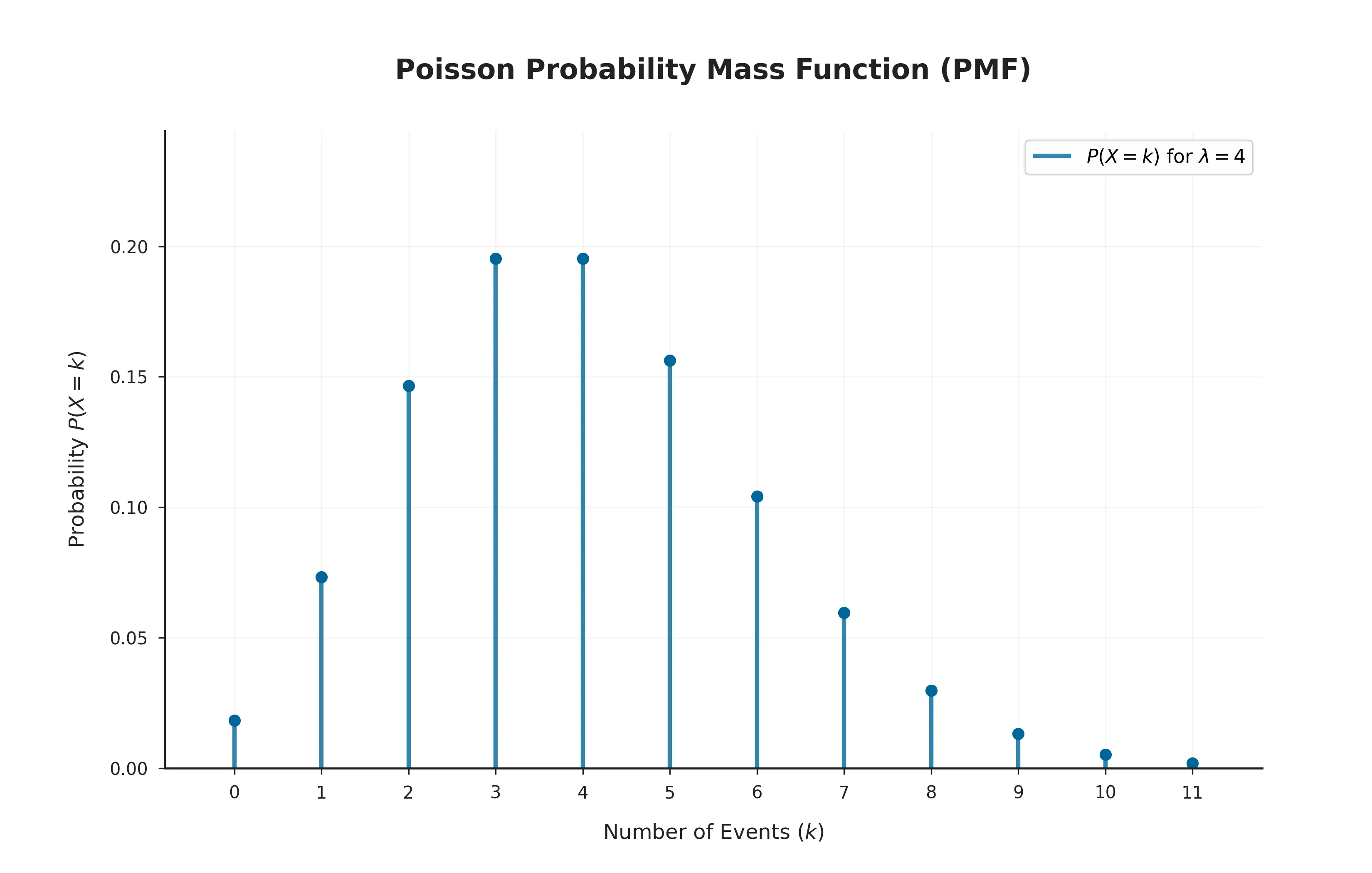
The probability mass function (PMF) of a Poisson distribution, which gives the probability of observing exactly \( k \) events in the interval, is:

Here \( \lambda > 0 \) is the rate parameter, the average number of events expected in the interval, \( e \) is Euler's number, and \( k! \) is the factorial of \( k \). Unlike the binomial PMF, which is defined only up to a finite ceiling \( n \), the Poisson PMF assigns strictly positive probability to every non-negative integer \( k \), no matter how large, though that probability shrinks rapidly toward zero once \( k \) grows well beyond \( \lambda \).

The formula falls out of the binomial PMF taken to its limit: substituting \( p = \lambda/n \) into \( \binom{n}{k}p^k(1-p)^{n-k} \) and letting \( n \to \infty \) causes the binomial coefficient and the \( (1-p)^{n-k} \) term to combine into \( e^{-\lambda} \), leaving exactly \( \lambda^k e^{-\lambda}/k! \) (see Binomial Origin & Normal Approximation for the full derivation). As with any valid PMF, the probabilities across all possible counts sum to exactly \( 1 \), which follows from recognizing the sum \( \sum_{k=0}^{\infty} \lambda^k/k! \) as the Taylor series for \( e^{\lambda} \).

Notation & Parameters

A Poisson distribution with rate \( \lambda \) is written compactly as:

read as "\( X \) follows a Poisson distribution with rate \( \lambda \)." Several conventions and constraints apply:

• \( \lambda \) must satisfy \( \lambda > 0 \); it represents both the average rate of events over the interval in question and, as shown in Core Properties, the distribution's mean and variance simultaneously.
• The support of the distribution — the set of values \( X \) can take — is the entire set of non-negative integers \( \{0, 1, 2, \ldots\} \), with no finite upper bound. This distinguishes it from the binomial distribution, whose support is capped at \( n \), while still keeping it discrete, unlike continuous distributions such as the normal distribution.
• \( \lambda \) is always tied to a specific interval of time, space, area, or volume. A rate of "\( 3 \) emails per hour" is a different parameter from "\( 3 \) emails per day" even though the underlying process is the same; scaling the interval scales \( \lambda \) proportionally, a property formalized in The Poisson Process.
• Some texts use \( \mu \) instead of \( \lambda \) for the rate parameter, particularly in applications framed around counts rather than rates, but the two notations refer to the identical distribution.

Core Properties

The Poisson distribution's defining mathematical signature is that a single parameter, \( \lambda \), simultaneously governs its mean, its variance, and — through the closed forms below — its skewness and kurtosis as well.

Mean (Expected Value)

The expected value of a Poisson random variable is exactly its rate parameter:

This matches the intuitive reading of \( \lambda \) as "the average number of events per interval," and is the reason \( \lambda \) can be estimated directly as a sample average from observed counts (see Estimating \( \lambda \) from Data).

Variance

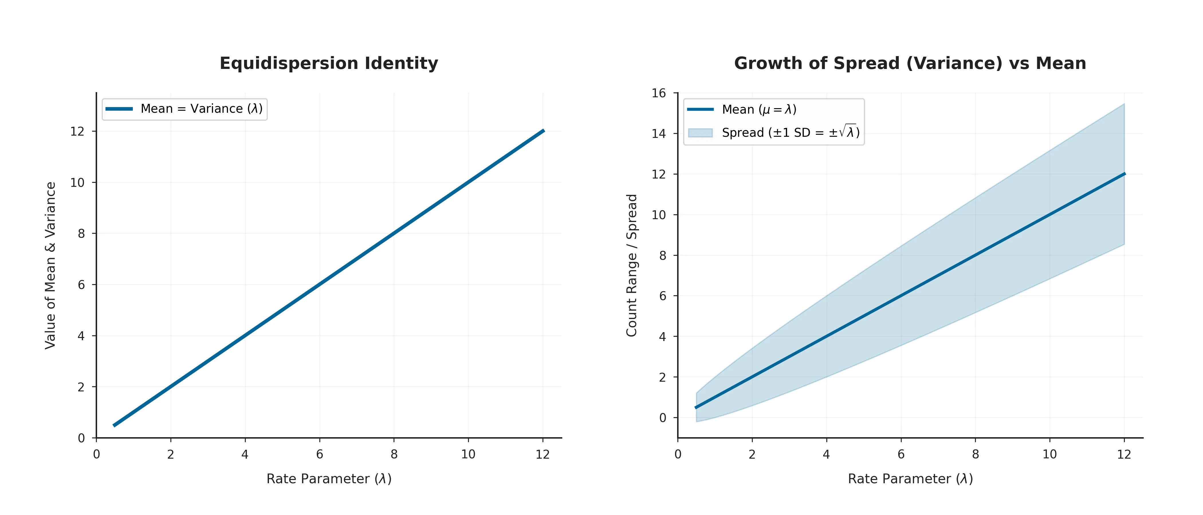
The variance of a Poisson random variable is, remarkably, also equal to \( \lambda \):

This equality of mean and variance — sometimes called the equidispersion property — is the single most distinctive feature of the Poisson distribution, and is frequently used as a diagnostic: if observed count data has a sample variance noticeably larger than its sample mean (overdispersion), a plain Poisson model is likely inadequate, and an alternative such as the negative binomial distribution is generally preferred (see Related Distributions).

Skewness

Skewness measures the asymmetry of a distribution. For a Poisson distribution it is:

The Poisson distribution is always positively (right) skewed for any finite \( \lambda \), since counts are bounded below by \( 0 \) but unbounded above. The skewness shrinks toward \( 0 \) as \( \lambda \) grows, meaning the distribution becomes progressively more symmetric for larger rates, which is what underlies the normal approximation discussed below.

Kurtosis

Kurtosis describes the shape of a distribution's tails relative to its center. For a Poisson distribution, the excess kurtosis is:

Like the skewness, the excess kurtosis is always positive and decreases toward \( 0 \) as \( \lambda \) increases, reinforcing that a Poisson distribution with a large rate looks increasingly bell-shaped and normal-like, while a Poisson distribution with a small rate is noticeably skewed and heavy in its right tail relative to a normal curve of the same variance.

Mode

The mode — the most probable count — is \( \lfloor \lambda \rfloor \) (the greatest integer less than or equal to \( \lambda \)) whenever \( \lambda \) is not itself an integer. When \( \lambda \) is a positive integer, the distribution is bimodal, with \( \lambda - 1 \) and \( \lambda \) equally probable. Because the mean \( \lambda \) can be any positive real number while the mode is restricted to integers, the two generally do not coincide exactly, mirroring the same mean/mode distinction seen in the Bernoulli and binomial distributions.

Shape as \( \lambda \) Varies

A single parameter controls every aspect of the Poisson distribution's shape, so tracing how the PMF deforms as \( \lambda \) increases builds most of the intuition needed before moving to formal approximations.

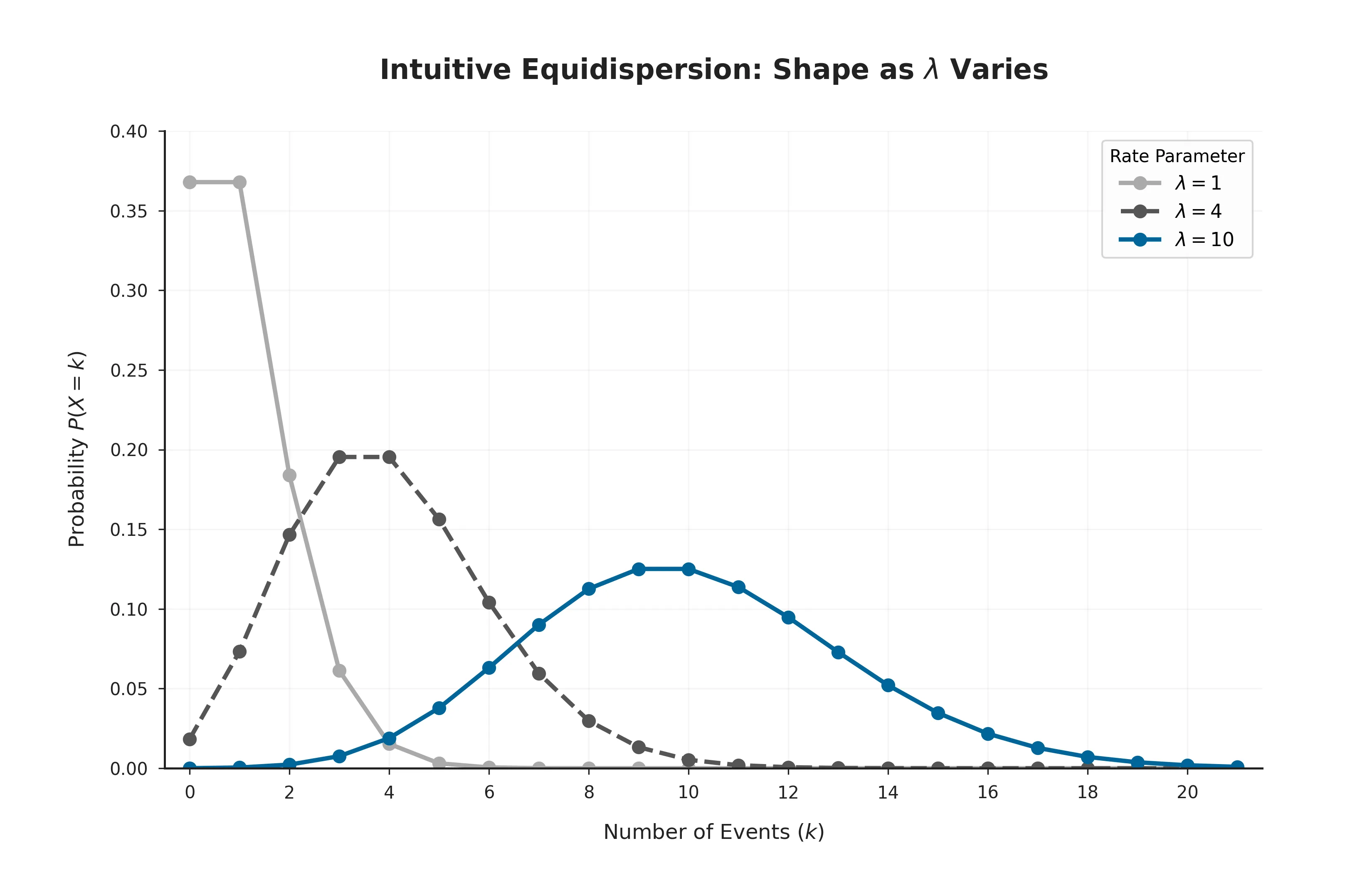
• Small \( \lambda \) (below about 1) concentrates most of the probability mass on \( 0, 1, \) and \( 2 \), with a pronounced right skew — the "zero events is the most likely outcome" regime typical of genuinely rare occurrences.
• Moderate \( \lambda \) (roughly 2 to 10) produces a visibly asymmetric hump centered near \( \lambda \), still noticeably skewed but no longer dominated by the single value \( 0 \).
• Large \( \lambda \) (above about 10) produces a distribution that is nearly symmetric and bell-shaped, closely tracking a normal curve with matching mean and variance (see Binomial Origin & Normal Approximation).
• Throughout, the distribution's spread — its standard deviation \( \sqrt{\lambda} \) — grows more slowly than its mean \( \lambda \), so relative variability (the coefficient of variation \( 1/\sqrt{\lambda} \)) shrinks as the rate increases, a pattern common to many count-based processes.

Moments & Generating Functions

The moment generating function (MGF) of a Poisson random variable has a distinctively compact double-exponential form:

Differentiating \( M(t) \) and evaluating at \( t=0 \) recovers the mean \( \lambda \) and, with the second derivative, the variance \( \lambda \), matching the direct calculations in Core Properties. This same functional form is what makes the sum of independent Poisson variables itself Poisson (see Sums of Poisson Variables), since multiplying MGFs of this exponential shape simply adds their rate parameters.

The related probability generating function, more commonly used for discrete distributions, is:

and the characteristic function follows the same pattern, \( \varphi_X(t) = \exp\!\big(\lambda(e^{it}-1)\big) \). Every generating function of a Poisson variable collapses events at rate \( \lambda \) into a single exponential term, which is precisely why the distribution arises so cleanly as a limit of the binomial distribution's own generating functions (see Binomial Origin & Normal Approximation).

Cumulative Distribution Function

The cumulative distribution function (CDF), \( F(k) = P(X \le k) \), gives the probability that a Poisson variable takes a value at or below a given threshold. It is obtained by summing the PMF over all counts from \( 0 \) up to \( k \):

Because the Poisson distribution's support extends to infinity, this sum never terminates at a fixed upper index the way the binomial CDF does at \( n \); instead, the terms shrink rapidly for \( i \) well beyond \( \lambda \), so the CDF converges to \( 1 \) without ever being computed as a truly infinite sum in practice. Like any discrete distribution's CDF, \( F(k) \) is a right-continuous staircase with a jump of height \( P(X=k) \) at every non-negative integer \( k \), in contrast to the smooth S-curve of the normal distribution's CDF. In closed form, \( F(k) \) can also be written using the regularized incomplete gamma function, \( F(k) = Q(k+1, \lambda) \), a relationship statistical software exploits to evaluate Poisson probabilities without summing every term individually.

Worked Example

Suppose a small customer-support team receives an average of \( \lambda = 5 \) support tickets per hour, and ticket arrivals are well modeled as independent events at a constant rate. Let \( X \sim \operatorname{Poisson}(5) \) denote the number of tickets received in a given hour. What are the mean and standard deviation of \( X \), and what is the probability that exactly three tickets arrive in the next hour?

Step 1 — Mean: using \( E[X] = \lambda \) from Core Properties:

Step 2 — Variance and standard deviation: using \( \operatorname{Var}(X) = \lambda \):

Step 3 — Probability of exactly three tickets: using the PMF with \( k=3 \):

There is roughly a 14.0% chance that exactly three tickets arrive in the next hour. Notice that the mode of this distribution is \( 4 \) and \( 5 \) (both equally likely, since \( \lambda = 5 \) is an integer, per Core Properties), while the single most probable individual outcome still carries less than a sixth of the total probability — typical of a moderately spread Poisson distribution rather than a sharply peaked one.

Estimating \( \lambda \) from Data

In practice, \( \lambda \) is rarely known exactly and must be estimated from observed counts. Given \( n \) independent observations \( x_1, \ldots, x_n \) from the same Poisson process, the maximum likelihood estimate (MLE) of \( \lambda \) is simply the sample mean of the observed counts:

This estimator is unbiased, since \( E[\hat\lambda] = \lambda \), and its variance, \( \operatorname{Var}(\hat\lambda) = \lambda/n \), shrinks toward zero as more intervals are observed — the formal justification for pooling more data to estimate a rate more precisely. Because the mean and variance of a Poisson variable coincide, the sample variance of the observed counts provides a natural, independent check on the Poisson assumption itself: if it diverges sharply from the sample mean, the equidispersion property from Core Properties is likely violated.

A common companion to the point estimate \( \hat\lambda \) is a confidence interval built from the relationship between the Poisson distribution and the chi-squared distribution, or, for large observed counts, the simpler normal-approximation interval \( \hat\lambda \pm z_{\alpha/2}\sqrt{\hat\lambda/n} \), which relies on the same large-\( \lambda \) approximation discussed next.

Binomial Origin & Normal Approximation

The Poisson distribution's relationship with two other classical distributions runs in opposite directions: it is the limit of one and is itself approximated by the other.

Origin as a Binomial Limit

As introduced in the introduction, the Poisson distribution arises as the limiting case of a binomial distribution when \( n \to \infty \) and \( p \to 0 \) while their product stays fixed at \( \lambda = np \):

Intuitively, this describes splitting a fixed interval into an enormous number of vanishingly small sub-intervals, each of which independently contains an event with tiny probability \( p \) — the discrete count of successes across those \( n \) micro-trials converges exactly to the continuous-time Poisson count as the sub-intervals shrink. A common practical guideline treats the binomial-to-Poisson approximation as reasonable when \( n \ge 20 \) and \( p \le 0.05 \), consistent with the same threshold given from the binomial side on the binomial distribution page.

Normal Approximation

Going the other direction, once \( \lambda \) is reasonably large, the Poisson distribution is itself well approximated by a normal distribution with matching mean and variance, a consequence of the central limit theorem applied to a Poisson variable viewed as a sum of many small independent contributions:

A widely used rule of thumb treats this approximation as reasonable once \( \lambda \ge 10 \), matching the point in Shape as \( \lambda \) Varies where the skewness \( 1/\sqrt{\lambda} \) and excess kurtosis \( 1/\lambda \) both become small. As with the binomial normal approximation, a continuity correction of \( \pm 0.5 \) is often applied when using the normal curve to estimate a discrete Poisson probability such as \( P(X \le k) \).

The Poisson Process

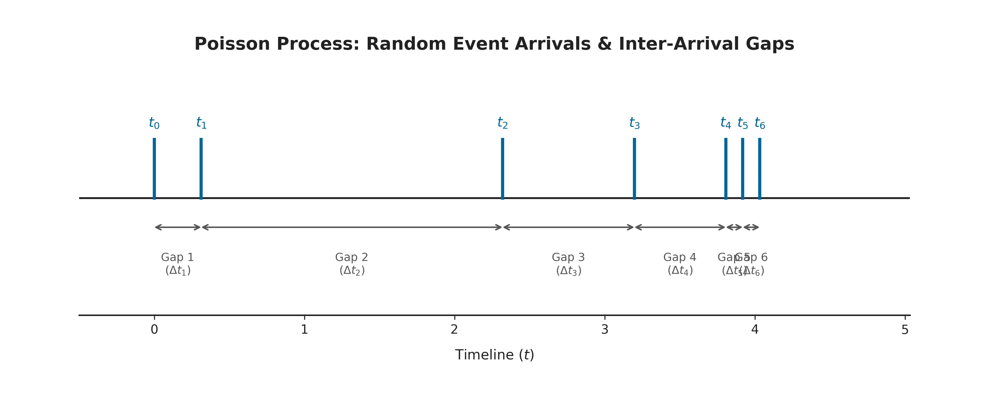
The Poisson distribution describes the count of events in a single fixed interval, but it is more commonly encountered as a snapshot of an underlying continuous-time model called the Poisson process: a stream of events occurring randomly over time (or space) such that

• events occur at a constant average rate \( \lambda \) per unit time (or, more generally, a rate that can vary, in the inhomogeneous case);
• the numbers of events in disjoint (non-overlapping) intervals are independent of one another; and
• events occur one at a time — the probability of two or more events happening at exactly the same instant is negligible.

Under these assumptions, the number of events falling within any interval of length \( t \) follows a \( \operatorname{Poisson}(\lambda t) \) distribution — scaling the interval scales the rate parameter proportionally, exactly as noted in Notation & Parameters. The complementary quantity, the waiting time between one event and the next, follows an exponential distribution with the same rate \( \lambda \); the two distributions are simply two different lenses — counts versus gaps — on the identical underlying random process. The time until the \( r \)-th event, summing \( r \) independent exponential gaps, follows a gamma distribution

Sums of Poisson Variables

The Poisson distribution has a clean and unrestricted closure property, cleaner even than the binomial distribution's closure under addition: if \( X_1 \sim \operatorname{Poisson}(\lambda_1) \) and \( X_2 \sim \operatorname{Poisson}(\lambda_2) \) are independent, their sum is again Poisson, with the two rates simply adding — no matching-parameter restriction is required:

This follows directly from the moment generating function in Moments & Generating Functions: multiplying \( \exp(\lambda_1(e^t-1)) \) and \( \exp(\lambda_2(e^t-1)) \) simply adds the exponents, producing the MGF of a \( \operatorname{Poisson}(\lambda_1+\lambda_2) \) variable. This property extends to any finite number of independent Poisson variables, and is the formal justification for aggregating separately measured rates — combining ticket counts from two support channels, or combining arrival counts from two intersections — into a single overall Poisson count.

Related Distributions

The Poisson distribution sits at the center of a web of closely related distributions, each obtained by varying one of its defining assumptions:

• Binomial distribution — the Poisson distribution is its limiting case as \( n \to \infty \) and \( p \to 0 \) with \( np = \lambda \) held fixed (see Binomial Origin & Normal Approximation).
• Exponential distribution — describes the waiting time between consecutive events in the same Poisson process that produces Poisson-distributed counts.
• Gamma distribution — describes the waiting time until the \( r \)-th event in a Poisson process, generalizing the exponential distribution to multiple events.
• Negative binomial distribution — a common remedy when count data is overdispersed (sample variance exceeds the sample mean), obtained by letting the Poisson rate \( \lambda \) itself vary randomly according to a gamma distribution (a Poisson-gamma mixture).
• Normal distribution — approximates the Poisson distribution well once \( \lambda \) is large, per Binomial Origin & Normal Approximation.
• Zero-inflated Poisson distribution — used when observed data contains more zero counts than a plain Poisson model would predict, mixing a Poisson component with an extra point mass at zero.
• Multinomial distribution — when a total Poisson count is split across several categories according to fixed proportions, the counts within each category, conditional on the total, follow a multinomial distribution.

Generating Poisson Random Numbers

Several algorithms exist for drawing a random sample from a Poisson\( (\lambda) \) distribution, with the right choice depending on how large \( \lambda \) is.

Knuth's algorithm is the simplest conceptually, and exploits the Poisson process's connection to the exponential distribution: repeatedly multiply uniform draws together until their running product falls below \( e^{-\lambda} \), and return the number of draws taken minus one. This works because each uniform draw corresponds to simulating one exponential inter-arrival gap, and the count of gaps that fit within a unit interval is exactly the Poisson count for that interval.

1. Set \( L = e^{-\lambda} \), \( k = 0 \), and \( p = 1 \).
2. Draw \( U \sim \operatorname{Uniform}(0,1) \), set \( p = p \times U \), and increment \( k \) by 1.
3. If \( p > L \), repeat step 2; otherwise return \( k - 1 \) as the Poisson draw.

This direct approach is simple but becomes slow for large \( \lambda \), since it requires roughly \( \lambda \) uniform draws per Poisson sample. Statistical software instead switches to faster methods for large \( \lambda \) — such as rejection sampling calibrated against the normal approximation, or table-lookup and transformation algorithms — that avoid the linear-time cost. In practice, these details are handled internally: for example, NumPy's numpy.random.poisson(lam) and SciPy's scipy.stats.poisson.rvs(mu) both return draws from a Poisson\( (\lambda) \) distribution without requiring any of the underlying algorithm to be implemented by hand.

A Short History

The distribution takes its name from the French mathematician Siméon Denis Poisson (1781–1840), who introduced it in his 1837 work Recherches sur la probabilité des jugements en matière criminelle et en matière civile ("Research on the Probability of Judgments in Criminal and Civil Matters"). Poisson derived the distribution as the limiting case of the binomial distribution for large \( n \) and small \( p \), extending the earlier work on binomial probabilities by Jacob Bernoulli and Abraham de Moivre to the regime of rare events (see A Short History on the binomial distribution page).

The distribution remained a relatively minor mathematical curiosity for decades until Ladislaus Bortkiewicz gave it its first celebrated real-world application in his 1898 book Das Gesetz der kleinen Zahlen ("The Law of Small Numbers"), famously showing that the annual number of Prussian cavalry soldiers kicked to death by horses fit a Poisson distribution remarkably well. This example, still cited today as an archetypal illustration of a Poisson-distributed rare event, helped establish the distribution as the standard tool for modeling counts of independent, low-probability occurrences, and it went on to become foundational to queueing theory through the early 20th-century work of Agner Krarup Erlang on telephone call arrivals.

Where It Shows Up

Any scenario reducible to "count how many independent, rare events happen in a fixed interval" is, in principle, Poisson. A selection of concrete examples across statistics, computing, and machine learning:

• Call centers and queueing systems — the number of calls, customer arrivals, or service requests in a fixed time window is the textbook Poisson application, underlying most queueing theory models.
• Web and network traffic — the number of requests hitting a server, or packets arriving at a router, in a fixed interval is commonly modeled as Poisson, informing capacity planning and load-testing.
• Insurance and actuarial science — the number of claims filed against a policy (or pool of policies) in a given year is a standard Poisson count, central to collective risk models.
• Poisson regression — a generalized linear model that predicts a Poisson- distributed count response (number of accidents, number of purchases) as a function of input features via a log link, widely used across epidemiology, economics, and applied machine learning.
• Natural language processing — the number of times a given word or n-gram appears in a fixed-length document is frequently approximated as Poisson, underlying some classical text-frequency and topic models.
• Genomics and radioactive decay — the number of mutations along a fixed length of DNA, or the number of radioactive decay events detected in a fixed time window, are classic physical and biological examples of Poisson counts.
• Manufacturing defect counts — the number of defects found on a fixed area of material (a roll of fabric, a sheet of glass) is commonly modeled as Poisson in statistical process control.
• Astronomy — the number of photons detected by a sensor in a fixed exposure time is modeled as Poisson, which is why "photon shot noise" in imaging follows Poisson statistics.

The Poisson model is occasionally misapplied when its core assumptions — a constant rate and independence between events — are violated: events that cluster together (an outage causing a burst of support tickets, contagion effects in claims data) typically produce overdispersion, where the negative binomial distribution or other mixture models are generally more appropriate than a plain Poisson assumption (see Related Distributions).

Frequently Asked Questions

• What is a Poisson distribution in simple terms? +
  It is the probability distribution of the number of times a rare, independent event occurs in a fixed interval of time or space, given that the events happen at a known constant average rate lambda and independently of the time since the last event.
• What is the difference between a Poisson distribution and a binomial distribution? +
  A binomial distribution counts successes in a fixed number of discrete trials n with success probability p. A Poisson distribution counts events over a continuous interval with an average rate lambda, and arises as the limit of a binomial distribution as n grows large and p shrinks such that np stays fixed at lambda.
• What are the mean and variance of a Poisson distribution? +
  For a Poisson random variable X with rate parameter lambda, both the mean and the variance equal lambda: E[X] = lambda and Var(X) = lambda. This equality of mean and variance is the distribution's defining signature.
• Why does the Poisson distribution matter in machine learning and statistics? +
  It is the standard model for count data - website visits, insurance claims, word occurrences, network arrivals - and underlies Poisson regression, the Poisson loss function used in count-prediction models, and generalized linear models with a log link for non-negative integer outcomes.
• What is the relationship between the Poisson distribution and the exponential distribution? +
  In a Poisson process, the number of events in a fixed interval follows a Poisson distribution, while the waiting time between consecutive events follows an exponential distribution with rate lambda; the two distributions describe the same underlying process from two different angles - counts versus gaps.
• When can the Poisson distribution be approximated by a normal distribution? +
  A common rule of thumb is that the normal approximation, X approximately Normal(lambda, lambda), becomes reasonable once lambda is at least 10, since the Poisson distribution grows increasingly symmetric and bell-shaped as its rate increases.
• Is the Poisson distribution discrete or continuous? +
  It is discrete: the random variable can take only non-negative integer values 0, 1, 2, and so on without any upper bound, so probability is described by a probability mass function rather than a probability density function.
• What distributions are related to the Poisson distribution? +
  The Poisson distribution is the small-p, large-n limit of the binomial distribution, the sum of independent Poisson variables is itself Poisson, the exponential and gamma distributions describe the waiting times between Poisson events, the negative binomial distribution generalizes it to allow overdispersion, and the normal distribution approximates it for large lambda.