
Bernoulli Distribution Explained
What Is a Bernoulli Distribution?
In probability theory and statistics, the Bernoulli distribution, named after the Swiss mathematician Jacob Bernoulli, is the discrete probability distribution of a random variable that takes exactly one of two possible values: \( 1 \), conventionally called success, with probability \( p \), and \( 0 \), called failure, with probability \( 1-p \). It is the simplest possible probability distribution over a random outcome, and is the fundamental building block for modeling any yes/no, true/false, or on/off event — a coin flip, a single click on an advertisement, whether a patient responds to a treatment, or a single bit in a message. See the formula below for the precise mathematical definition.
A single instance of a Bernoulli-distributed experiment is called a Bernoulli trial. The distribution is fully described by one parameter, the success probability \( p \), which makes it both the simplest member of the discrete distribution family and, not coincidentally, the starting point from which several other well-known distributions — the binomial, geometric, and negative binomial among them — are built by repeating or counting Bernoulli trials (see Related Distributions).
The Formula
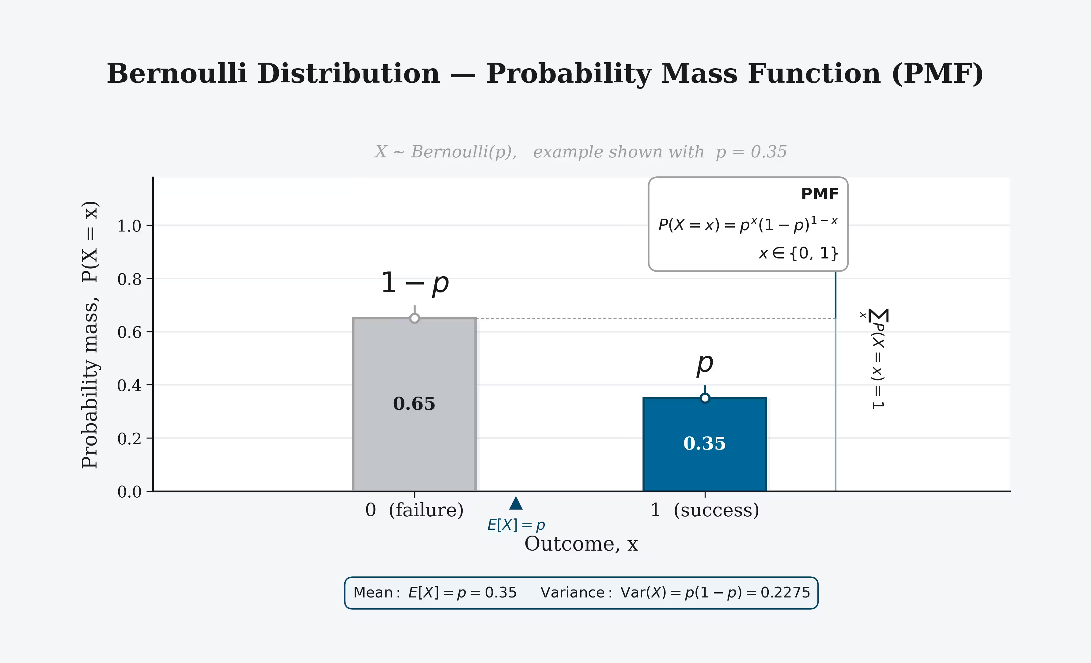
The probability mass function (PMF) of a Bernoulli distribution, which gives the probability of each of the two possible outcomes, is:
\[ P(X = x) = \begin{cases} p & \text{if } x = 1 \\ 1-p & \text{if } x = 0 \end{cases} \]Here \( p \) is the success probability, the single parameter that fully specifies the distribution. This piecewise definition is commonly written more compactly as a single closed-form expression, valid for \( x \in \{0, 1\} \):
\[ P(X = x) = p^x (1-p)^{1-x} \]The two forms are equivalent: substituting \( x=1 \) collapses the exponent on \( (1-p) \) to zero, leaving \( p \); substituting \( x=0 \) collapses the exponent on \( p \) to zero, leaving \( 1-p \). Unlike the normal distribution's density, which is defined over a continuum of values, the Bernoulli PMF assigns probability directly to just two discrete outcomes, and the two probabilities always sum to \( 1 \), since success and failure are the only possibilities.
Notation & Parameters
A Bernoulli distribution with success probability \( p \) is written compactly as:
\[ X \sim \operatorname{Bernoulli}(p) \quad \text{or equivalently} \quad X \sim \operatorname{Bern}(p) \]read as "\( X \) follows a Bernoulli distribution with success probability \( p \)." Several conventions and constraints apply:
- \( p \) must satisfy \( 0 \le p \le 1 \), since it is itself a probability. Some texts require the strict inequality \( 0 < p < 1 \), treating \( p=0 \) and \( p=1 \) as degenerate edge cases where the outcome is certain rather than genuinely random.
- The support of the distribution — the set of values \( X \) can take — is the two-element set \( \{0, 1\} \), and nothing else. This makes the Bernoulli distribution discrete, in contrast to continuous distributions such as the normal or uniform distributions.
- The quantity \( q = 1-p \) is frequently used as shorthand for the failure probability, particularly in older texts and in combinatorics, where it simplifies expressions such as the binomial PMF (see Related Distributions).
- A Bernoulli random variable is often called an indicator variable when it is defined to take the value \( 1 \) exactly when some event \( A \) occurs and \( 0 \) otherwise, written \( X = \mathbb{1}_A \). In that framing, \( p = P(A) \) and \( E[X] = P(A) \), a identity used constantly throughout probability theory to convert between "the probability of an event" and "the expected value of an indicator."
Core Properties
Despite having only two possible outcomes, the Bernoulli distribution has a full set of the same descriptive properties — mean, variance, skewness, kurtosis — used to characterize any probability distribution, each with an unusually simple closed form.
Mean (Expected Value)
The expected value of a Bernoulli random variable is exactly its success probability:
\[ E[X] = 1 \cdot p + 0 \cdot (1-p) = p \]This is a direct consequence of the definition of expectation for a discrete variable: each outcome is weighted by its probability, and since the \( 0 \) outcome contributes nothing to the sum, the mean collapses to \( p \) alone. This identity is what allows \( p \) to be estimated directly as a sample average (see Estimating p from Data).
Variance
The variance measures how much the outcome is expected to deviate from the mean, and for a Bernoulli variable it has the compact form:
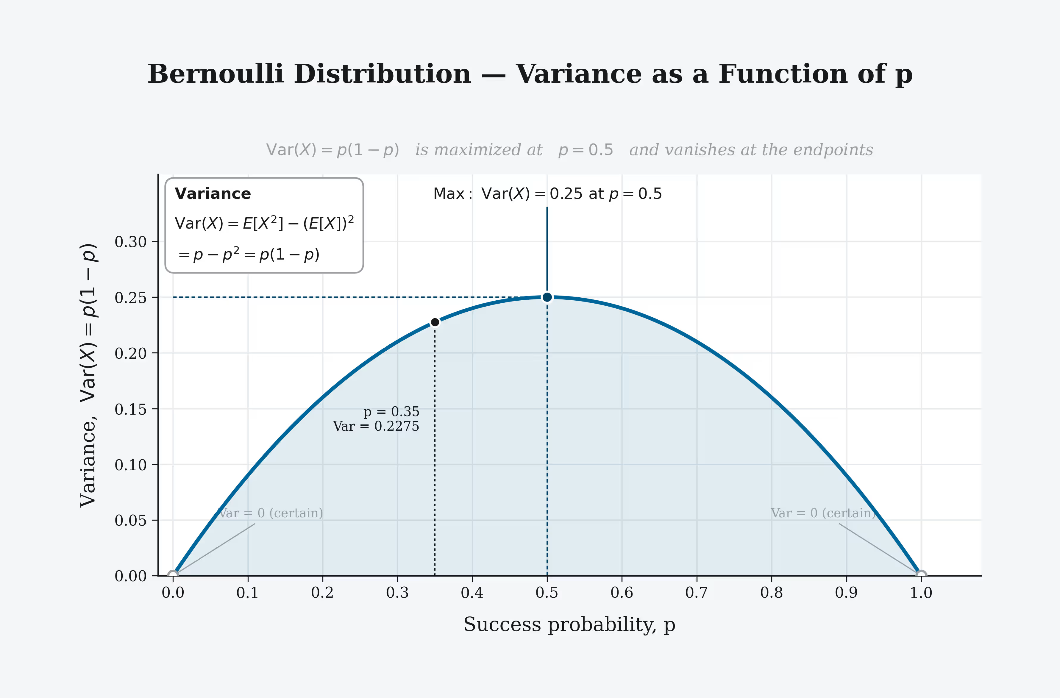
\[ \operatorname{Var}(X) = E[X^2] - (E[X])^2 = p - p^2 = p(1-p) \]Since \( X^2 = X \) whenever \( X \in \{0,1\} \) (both \( 0^2=0 \) and \( 1^2=1 \)), \( E[X^2] = E[X] = p \), which is what produces the simplification above. The variance \( p(1-p) \) is maximized at \( p=0.5 \), where it equals \( 0.25 \) — a fair coin flip is the "most random" possible Bernoulli trial — and shrinks toward \( 0 \) as \( p \) approaches either \( 0 \) or \( 1 \), where the outcome becomes nearly certain.
Skewness
Skewness measures the asymmetry of a distribution. For a Bernoulli distribution it is:
\[ \text{Skewness} = \frac{1-2p}{\sqrt{p(1-p)}} \]Unlike the normal distribution, which is always symmetric, a Bernoulli distribution is symmetric only at the single point \( p=0.5 \), where the skewness is exactly \( 0 \). For \( p < 0.5 \), the skewness is positive (failure, \( 0 \), is the far more common outcome, and the rare success sits like a right tail); for \( p > 0.5 \), it is negative. The magnitude of the skewness grows without bound as \( p \) approaches \( 0 \) or \( 1 \), reflecting an increasingly rare, increasingly "surprising" outcome on one side.
Kurtosis
Kurtosis describes the shape of a distribution's tails relative to its center. For a Bernoulli distribution, the excess kurtosis is:
\[ \text{Excess kurtosis} = \frac{1-6p(1-p)}{p(1-p)} = \frac{1}{p(1-p)} - 6 \]This is minimized at \( p=0.5 \), where it equals \( 4 - 6 = -2 \) — the lowest possible excess kurtosis of any distribution, discrete or continuous, a fact sometimes cited as a curiosity in the theory of moments. Away from \( p=0.5 \), the excess kurtosis grows rapidly, since \( p(1-p) \) shrinks toward zero and appears in the denominator.
Mode
The mode — the most probable outcome — is \( 1 \) whenever \( p > 0.5 \), \( 0 \) whenever \( p < 0.5 \), and both \( 0 \) and \( 1 \) are equally probable (a bimodal case) exactly when \( p = 0.5 \). Unlike the normal distribution, where mean, median, and mode coincide, a Bernoulli variable's mean \( p \) generally does not equal its mode at all, since the mean can take any value in \( [0,1] \) while the mode is restricted to \( \{0, 1\} \) (or both).
Moments & Generating Functions
Because a Bernoulli variable satisfies \( X^k = X \) for every positive integer \( k \) (raising \( 0 \) or \( 1 \) to any power leaves it unchanged), all of its raw moments collapse to the same value:
\[ E[X^k] = p \qquad \text{for every } k = 1, 2, 3, \ldots \]This is a distinctive feature of two-point distributions: unlike continuous distributions, where each successive moment typically carries new information, every raw moment of a Bernoulli variable is simply \( p \) again.
The moment generating function (MGF) is a single function that encodes every moment of a distribution at once. For a Bernoulli distribution with success probability \( p \), it is:
\[ M(t) = E\left[e^{tX}\right] = (1-p) + p\,e^{t} \]since the sum defining the expectation has only two terms, one for each possible outcome. Differentiating \( M(t) \) and evaluating at \( t=0 \) recovers the mean and, together with the second derivative, the variance, matching the direct calculations above.
The related characteristic function is \( \varphi_X(t) = E[e^{itX}] = (1-p) + p\,e^{it} \), and the probability generating function, more commonly used for discrete distributions, is \( G(z) = E[z^X] = (1-p) + pz \) — a straight line in \( z \), the simplest possible form a probability generating function can take.
Finally, the entropy of a Bernoulli distribution, measured in bits (using \( \log_2 \)), is given by the binary entropy function:
\[ H(p) = -p\log_2 p - (1-p)\log_2(1-p) \]Entropy quantifies the average uncertainty, in bits, of the outcome of one trial. It is maximized at \( p=0.5 \), where \( H(0.5)=1 \) bit — a fair coin flip carries exactly one bit of information, the theoretical basis of the bit as a unit of information — and falls to \( 0 \) as \( p \) approaches either \( 0 \) or \( 1 \), where the outcome becomes certain and no information is gained by observing it.
Cumulative Distribution Function
The cumulative distribution function (CDF), \( F(x) = P(X \le x) \), gives the probability that a Bernoulli variable is at or below a given threshold. Because the distribution has only two support points, the CDF is a simple step function:
\[ F(x) = \begin{cases} 0 & \text{if } x < 0 \\ 1-p & \text{if } 0 \le x < 1 \\ 1 & \text{if } x \ge 1 \end{cases} \]The graph rises from \( 0 \), jumps to height \( 1-p \) at \( x=0 \), stays flat until \( x=1 \), then jumps the rest of the way to \( 1 \). This staircase shape is characteristic of any discrete distribution's CDF, in contrast to the smooth S-curve of the normal distribution's CDF: there is no probability mass strictly between \( 0 \) and \( 1 \), so the function cannot rise smoothly through that gap.
Worked Example
Suppose an online advertisement is shown to a single visitor, and the probability that this particular visitor clicks it is known from historical data to be \( p = 0.04 \) (a 4% click-through rate). Let \( X \sim \operatorname{Bernoulli}(0.04) \) denote whether this visitor clicks (\( X=1 \)) or not (\( X=0 \)). What are the mean and standard deviation of \( X \), and what is the probability the visitor does not click?
Step 1 — Mean: using \( E[X] = p \) from Core Properties:
\[ E[X] = 0.04 \]Step 2 — Variance and standard deviation: using \( \operatorname{Var}(X) = p(1-p) \):
\[ \operatorname{Var}(X) = 0.04 \times 0.96 = 0.0384, \qquad \operatorname{SD}(X) = \sqrt{0.0384} \approx 0.196 \]Step 3 — Probability of no click: directly from the PMF, \( P(X=0) = 1-p \):
\[ P(X=0) = 1 - 0.04 = 0.96 \]There is a 96% chance this particular visitor does not click the advertisement. Note that even though the expected value \( 0.04 \) is a perfectly valid number, it is not itself a possible outcome of any single trial — a single visitor either clicks or does not, and \( 0.04 \) only describes the long-run average click rate across many such visitors (see Sums of Bernoulli Variables for what happens when many trials are combined).
Estimating p from Data
In practice, \( p \) is rarely known exactly and must be estimated from observed data. Given \( n \) independent Bernoulli trials \( X_1, X_2, \ldots, X_n \), all sharing the same unknown success probability \( p \), the maximum likelihood estimate (MLE) of \( p \) is simply the sample proportion of successes:
\[ \hat{p} = \frac{1}{n}\sum_{i=1}^{n} X_i = \frac{\text{number of successes}}{n} \]This estimator is unbiased, since \( E[\hat p] = p \), and its own variance is \( \operatorname{Var}(\hat p) = p(1-p)/n \), which shrinks toward zero as more trials are observed — the formal justification for why larger samples give more reliable estimates of a success rate.
In a Bayesian setting, the natural conjugate prior for \( p \) is the Beta distribution: starting from a \( \operatorname{Beta}(\alpha, \beta) \) prior and observing \( k \) successes in \( n \) trials updates it to a \( \operatorname{Beta}(\alpha+k,\ \beta+n-k) \) posterior, a closed-form update that requires no numerical integration (see Related Distributions).
Sums of Bernoulli Variables
Unlike the normal distribution, which is closed under addition, summing independent Bernoulli variables does not produce another Bernoulli distribution — the sum can exceed \( 1 \), which is outside the Bernoulli support. Instead, if \( X_1, \ldots, X_n \) are independent and identically distributed \( \operatorname{Bernoulli}(p) \) variables, their sum follows a binomial distribution:
\[ S_n = \sum_{i=1}^{n} X_i \sim \operatorname{Binomial}(n, p) \]counting the total number of successes across the \( n \) trials, with probability mass function \( P(S_n=k) = \binom{n}{k}p^k(1-p)^{n-k} \). By linearity of expectation and independence of variance, the mean and variance scale directly:
\[ E[S_n] = np, \qquad \operatorname{Var}(S_n) = np(1-p) \]As \( n \) grows large, the shape of the binomial distribution approaches a normal bell curve (a consequence of the central limit theorem), which is the basis of the normal approximation to the binomial commonly used when \( n \) is large and \( p \) is not too close to \( 0 \) or \( 1 \). This same summing logic — treating a count as a sum of many small binary indicator variables — is one of the most frequently reused patterns in applied probability.
Generating Bernoulli Random Numbers
Because a Bernoulli variable takes only two values, generating one is the simplest possible case of random variate generation, and reduces directly to a single draw from a uniform distribution:
- Draw \( U \sim \operatorname{Uniform}(0,1) \) from a pseudo-random number generator.
- Set \( X = 1 \) if \( U < p \), and \( X = 0 \) otherwise.
This is a special case of inverse transform sampling: the interval \( [0,1) \) is split into a sub-interval of length \( p \) (mapped to success) and length \( 1-p \) (mapped to failure), and the uniform draw simply determines which side it lands on. Every other method of generating discrete random variables — the binomial, geometric, and categorical distributions among them — ultimately reduces to repeated applications of this same comparison.
Standard scientific computing libraries provide this directly rather than requiring it to be implemented by hand: for example, NumPy's numpy.random.binomial(1, p) or, more directly, SciPy's scipy.stats.bernoulli.rvs(p) both return draws from a Bernoulli\( (p) \) distribution using this comparison internally.
A Short History
The distribution takes its name from Jacob Bernoulli (1654–1705), a member of the prolific Bernoulli family of Swiss mathematicians, whose posthumously published 1713 work Ars Conjectandi ("The Art of Conjecturing") laid much of the early groundwork for probability theory. Bernoulli studied repeated trials with two outcomes — what would later be called Bernoulli trials — primarily as a route to deriving the binomial distribution and, within the same work, an early version of the law of large numbers, which formalizes the intuition that a sample proportion converges to the true probability \( p \) as the number of trials grows.
The term "Bernoulli distribution" itself, referring to the single-trial case in isolation, came into standard use considerably later, as 20th-century probability theory was formalized on rigorous measure-theoretic foundations by figures such as Andrey Kolmogorov. Within that framework, the Bernoulli distribution serves as the canonical minimal example of a random variable, and Bernoulli trials underpin the construction of more general stochastic processes, including random walks and the earliest models of what became modern information theory.
Where It Shows Up
Any scenario reducible to a single binary outcome is, in principle, a Bernoulli trial. A selection of concrete examples across statistics, computing, and machine learning:
- Binary classification — the label predicted for a single example (spam vs. not spam, fraud vs. not fraud) is modeled as a Bernoulli outcome.
- Logistic regression — models the success probability \( p \) of a Bernoulli outcome as a function of input features, with model fitting driven by the Bernoulli likelihood.
- Binary cross-entropy loss — the standard loss function for binary classifiers in machine learning is precisely the negative log-likelihood of a Bernoulli distribution.
- Bernoulli naive Bayes — a text-classification model in which each word's presence or absence in a document is treated as an independent Bernoulli variable.
- Dropout regularization — during neural network training, each unit is independently kept or dropped according to a Bernoulli draw.
- A/B testing — whether an individual visitor converts, clicks, or completes a purchase is modeled as a Bernoulli outcome, with the two variants compared on their estimated success probabilities.
- Quality control — whether a single manufactured unit passes or fails inspection is a Bernoulli outcome, aggregated into a binomial count across a production run.
- Reliability engineering — whether a single component functions or fails within a given time window is frequently modeled as Bernoulli, particularly in discrete-time reliability models.
- Information theory — a single binary digit (bit) generated by a memoryless binary source is modeled as a Bernoulli variable, with the source's entropy given by the binary entropy function (see Moments & Generating Functions).
Bernoulli models are occasionally misapplied to outcomes that are not truly independent or not truly identically distributed across trials — repeated measurements on the same subject, for instance, often violate independence. When trials are correlated or when the success probability itself varies, extensions such as the Beta-binomial distribution or hierarchical (mixed-effects) models are generally more appropriate than a plain Bernoulli/binomial assumption.
Frequently Asked Questions
- It is the probability distribution of a single trial that has only two possible outcomes, usually labeled success (1) and failure (0), where success occurs with a fixed probability p and failure occurs with probability 1 - p.
- A Bernoulli distribution describes the outcome of a single trial with two possible outcomes. A binomial distribution describes the total number of successes across n independent Bernoulli trials with the same success probability p; a Bernoulli distribution is the special case of a binomial distribution with n = 1.
- For a Bernoulli random variable X with success probability p, the mean is E[X] = p and the variance is Var(X) = p(1 - p).
- It is the natural likelihood model for binary classification, underlies logistic regression and the binary cross-entropy loss function, and appears in Bernoulli naive Bayes, dropout regularization, and any setting where an outcome is modeled as a single yes/no event.
- The skewness is (1 - 2p) / sqrt(p(1-p)), which is zero only when p = 0.5 and grows in magnitude as p moves toward 0 or 1; the excess kurtosis is (1 - 6p(1-p)) / (p(1-p)), which is always positive except at p = 0.5.
- Given n independent Bernoulli observations, the maximum likelihood estimate of p is simply the sample proportion of successes, i.e. the number of 1s divided by n.
- It is discrete: the random variable can take only two values, 0 and 1, so probability is described by a probability mass function rather than a probability density function.
- The binomial distribution is a sum of n independent Bernoulli trials, the geometric distribution counts the number of Bernoulli trials until the first success, the categorical distribution generalizes it to more than two outcomes, and the beta distribution is its conjugate prior in Bayesian inference.