
Independent Samples t-test: When, Why, and How to Use It
Introduction
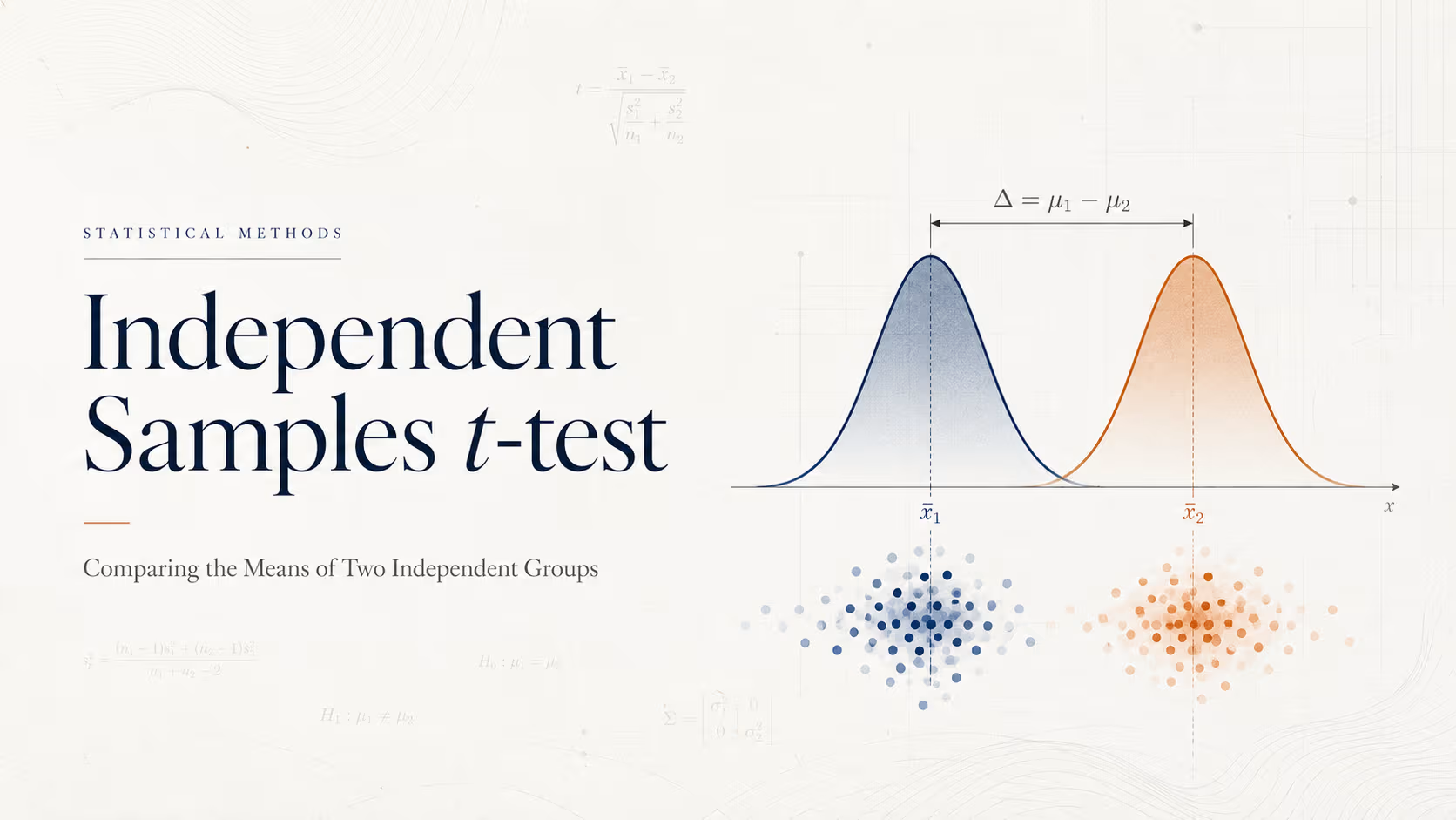
The independent samples t-test (also called the two-sample t-test or unpaired t-test) checks whether the means of two separate, unrelated groups are statistically significantly different. If you have ever compared a treatment group against a control group, version A against version B with two different sets of users, or men against women on some outcome-this is usually the test you are looking for.
By the end of this article you will be able to state exactly when an independent samples t-test applies, compute one completely by hand on two different worked examples, know when to switch to Welch's correction, interpret the result correctly alongside an effect size and confidence interval, and run the same test in three lines of Python with scipy.stats.ttest_ind.
What Is an Independent Samples t-test?
The independent samples t-test compares the means of two groups made up of different, unrelated subjects. Unlike a before-and-after design, there is no natural link between an observation in group 1 and any particular observation in group 2-each group simply contributes its own sample of values, and the test asks: on average, is the difference between the two group means larger than we would expect from random sampling variation alone?
It exists because comparing two unrelated groups is one of the most common questions in experimental and observational research. Because the two samples share no link between individual observations, the test must account for variability within each group as well as the gap between the two group means-which is why, unlike the paired t-test, it cannot simply collapse the data down to a single column of differences.
When to Use It
Use an independent samples t-test when you are comparing two separate groups of different subjects-a treatment group and a control group, users assigned to version A versus version B, or any split where each subject belongs to exactly one of the two groups. The key requirement: the two samples are independent-no subject appears in both groups, and no natural pairing links an observation in one group to a specific observation in the other.
| Scenario | Group 1 | Group 2 |
|---|---|---|
| Clinical trial | Outcome, drug group | Outcome, placebo group |
| A/B testing (different users) | Conversion rate, version A users | Conversion rate, version B users |
| Teaching method comparison | Test scores, Method 1 class | Test scores, Method 2 class |
| Gender comparison | Salary, male employees | Salary, female employees |
| Manufacturing quality | Defect rate, Supplier A | Defect rate, Supplier B |
| Diet comparison | Weight loss, Diet A group | Weight loss, Diet B group |
Key Assumptions
- Independent/unrelated samples. Each observation belongs to exactly one group, and there is no meaningful link between an observation in group 1 and any specific observation in group 2.
- Data are approximately normal within each group. Especially important with small samples; less critical as group sizes grow, thanks to the Central Limit Theorem.
- Continuous data. Scores, measurements, or any interval/ratio-scale variable-not categories.
- Homogeneity of variance (for Student's version). The two groups should have roughly equal variances. When this is not true, use Welch's t-test instead.
- No major outliers. Since the test relies on group means, a few extreme values in either group can distort the result.
Hypotheses
The independent samples t-test formally tests whether the two population means (\( \mu_1 \) and \( \mu_2 \)) are equal:
- Null Hypothesis (\( H_0 \)): the two population means are equal (\( \mu_1 = \mu_2 \))-i.e., there is no real difference between the groups.
- Alternative Hypothesis (\( H_1 \)): the two population means are not equal (\( \mu_1 \neq \mu_2 \))-i.e., there is a real difference.
(For one-tailed tests, \( H_1 \) can instead state one mean is specifically greater than or less than the other, depending on the direction being tested-for example \( \mu_1 > \mu_2 \) if you only care whether group 1 scored higher.)
The Formula, Explained
For two independent groups of size \( n_1 \) and \( n_2 \), with sample means \( \bar{x}_1, \bar{x}_2 \) and sample variances \( s_1^2, s_2^2 \), assuming equal population variances (Student's t-test), the test statistic is:
\[ t = \frac{\bar{x}_1 - \bar{x}_2}{s_p \sqrt{\dfrac{1}{n_1} + \dfrac{1}{n_2}}} \]where the pooled standard deviation \( s_p \) combines the variance of both groups, weighted by their degrees of freedom:
\[ s_p = \sqrt{\frac{(n_1 - 1)s_1^2 + (n_2 - 1)s_2^2}{n_1 + n_2 - 2}} \]This \( t \) value is compared against a Student's t-distribution with \( n_1 + n_2 - 2 \) degrees of freedom to obtain a p-value. Pooling the two variances into one shared estimate is what makes this the "equal variances" version of the test-if that assumption looks shaky, use Welch's t-test instead.
Welch's t-test (Unequal Variances)
When the two groups do not have similar variances-especially combined with unequal sample sizes-pooling the variances can distort the result. Welch's t-test avoids this by using each group's own variance separately, without pooling:
\[ t = \frac{\bar{x}_1 - \bar{x}_2}{\sqrt{\dfrac{s_1^2}{n_1} + \dfrac{s_2^2}{n_2}}} \]The degrees of freedom are no longer a simple \( n_1 + n_2 - 2 \); instead they are approximated with the Welch-Satterthwaite equation, which typically yields a non-integer value:
\[ df \approx \frac{\left(\dfrac{s_1^2}{n_1} + \dfrac{s_2^2}{n_2}\right)^2}{\dfrac{(s_1^2/n_1)^2}{n_1 - 1} + \dfrac{(s_2^2/n_2)^2}{n_2 - 1}} \]t.test()-recommend using Welch's version by default rather than testing for equal variances first and picking a formula based on the result. Worked Example 1: A Small Numerical Example by Hand
Suppose a researcher recruits two separate, unrelated groups of 5 adults each to test two different diets and records weight loss (in kg) after 8 weeks.
| Diet A (kg lost) | Diet B (kg lost) |
|---|---|
| 24 | 21 |
| 28 | 25 |
| 22 | 23 |
| 27 | 20 |
| 25 | 24 |
Step 1: Compute each group's mean and variance
\[ \bar{x}_1 = \frac{24+28+22+27+25}{5} = \frac{126}{5} = 25.2 \qquad \bar{x}_2 = \frac{21+25+23+20+24}{5} = \frac{113}{5} = 22.6 \]Sum of squared deviations from each mean: Diet A \( = 5.7 \times 4 = 22.8 \), so \( s_1^2 = 22.8/4 = 5.7 \). Diet B \( = 4.3 \times 4 = 17.2 \), so \( s_2^2 = 17.2/4 = 4.3 \).
\[ s_1^2 = 5.7, \quad s_1 \approx 2.3875 \qquad\qquad s_2^2 = 4.3, \quad s_2 \approx 2.0736 \]Step 2: Compute the pooled standard deviation
\[ s_p = \sqrt{\frac{(5-1)(5.7) + (5-1)(4.3)}{5 + 5 - 2}} = \sqrt{\frac{22.8 + 17.2}{8}} = \sqrt{5.0} \approx 2.2361 \]Step 3: Compute the t-statistic
\[ t = \frac{25.2 - 22.6}{2.2361 \sqrt{\tfrac{1}{5} + \tfrac{1}{5}}} = \frac{2.6}{2.2361 \times 0.6325} = \frac{2.6}{1.4142} \approx 1.838 \]Step 4: Compare against the critical value
With \( df = n_1 + n_2 - 2 = 8 \) and a two-tailed test at \( \alpha = 0.05 \), the critical value from the t-distribution table is \( t_{0.025, 8} = 2.306 \). Since our computed \( |t| = 1.838 \) is less than 2.306, we fail to reject \( H_0 \) at the 5% level-the corresponding two-tailed p-value works out to approximately 0.103, which is above 0.05.
Worked Example 2: Comparing Two Training Methods (Unequal Group Sizes)
Suppose 7 employees are trained with a new onboarding method and 6 different employees are trained with the old method. We want to know if the new method produced higher assessment scores. Note the group sizes are unequal-this is completely fine for an independent samples t-test.
| New Method (n=7) | Old Method (n=6) |
|---|---|
| 85 | 78 |
| 90 | 82 |
| 88 | 75 |
| 92 | 80 |
| 84 | 79 |
| 91 | 77 |
| 89 |
Step 1: Group means and variances
\[ \bar{x}_1 = \frac{85+90+88+92+84+91+89}{7} = \frac{619}{7} \approx 88.429 \qquad \bar{x}_2 = \frac{78+82+75+80+79+77}{6} = \frac{471}{6} = 78.5 \] \[ s_1^2 \approx 8.952, \quad s_1 \approx 2.992 \qquad\qquad s_2^2 = 5.9, \quad s_2 \approx 2.429 \]Step 2: Pooled standard deviation
\[ s_p = \sqrt{\frac{(7-1)(8.952) + (6-1)(5.9)}{7 + 6 - 2}} = \sqrt{\frac{53.71 + 29.5}{11}} = \sqrt{7.565} \approx 2.7505 \]Step 3: t-statistic
\[ t = \frac{88.429 - 78.5}{2.7505 \sqrt{\tfrac{1}{7} + \tfrac{1}{6}}} = \frac{9.929}{2.7505 \times 0.5563} = \frac{9.929}{1.5302} \approx 6.488 \]Step 4: Decision
With \( df = n_1 + n_2 - 2 = 11 \), the two-tailed critical value at \( \alpha = 0.05 \) is \( t_{0.025,11} = 2.201 \). Since \( 6.488 > 2.201 \), we reject \( H_0 \). The exact two-tailed p-value is approximately 0.000045, far below 0.05-the new onboarding method appears to have produced a statistically significant improvement.
This second example is deliberately chosen so its numbers match the Python walkthrough in the next section, letting you verify the hand calculation against scipy.stats.ttest_ind directly-including a check of whether Welch's correction changes the conclusion.
Effect Size (Cohen's d for Independent Samples)
A p-value tells you whether a difference is likely to be real; it says nothing about how large that difference is. For independent samples, the standard effect size is Cohen's d, computed by standardizing the difference between the two means by the pooled standard deviation:
\[ d = \frac{\bar{x}_1 - \bar{x}_2}{s_p} \]Using Worked Example 2: \( d = \dfrac{9.929}{2.7505} \approx 3.61 \). By Cohen's conventional benchmarks (\( d \approx 0.2 \) small, \( 0.5 \) medium, \( 0.8 \) large), a \( d \) of 3.61 is an extremely large effect-consistent with the very small p-value found above.
| Cohen's d | Interpretation |
|---|---|
| ~0.2 | Small effect |
| ~0.5 | Medium effect |
| ~0.8 | Large effect |
| 1.0+ | Very large effect |
Confidence Interval for the Mean Difference
A 95% confidence interval for \( \mu_1 - \mu_2 \) is often more informative than the p-value alone, since it shows the plausible range of the true difference in the original units:
\[ (\bar{x}_1 - \bar{x}_2) \pm t_{\alpha/2, \, df} \cdot s_p\sqrt{\frac{1}{n_1} + \frac{1}{n_2}} \]For Worked Example 2, with \( \bar{x}_1 - \bar{x}_2 = 9.929 \), \( s_p\sqrt{1/n_1 + 1/n_2} = 1.5302 \), and \( t_{0.025,11} = 2.201 \):
\[ 9.929 \pm 2.201 \times 1.5302 = 9.929 \pm 3.368 \]This gives a 95% CI of approximately [6.56, 13.30] points. Since the entire interval lies above zero, it agrees with the earlier rejection of \( H_0 \)-and gives a concrete, interpretable range for the likely true difference, rather than just a binary significant/not-significant verdict.
Python Example
You can run this test in one line using scipy.stats.ttest_ind:
from scipy import stats
import numpy as np

new_method = [85, 90, 88, 92, 84, 91, 89]
old_method = [78, 82, 75, 80, 79, 77]

# Student's t-test (assumes equal variances)
t_stat, p_value = stats.ttest_ind(new_method, old_method, equal_var=True)

print(f"t-statistic: {t_stat:.3f}")
print(f"p-value: {p_value:.6f}")

# Effect size: Cohen's d (pooled standard deviation)
n1, n2 = len(new_method), len(old_method)
var1, var2 = np.var(new_method, ddof=1), np.var(old_method, ddof=1)
pooled_sd = np.sqrt(((n1 - 1) * var1 + (n2 - 1) * var2) / (n1 + n2 - 2))
mean_diff = np.mean(new_method) - np.mean(old_method)
cohens_d = mean_diff / pooled_sd
print(f"Mean difference: {mean_diff:.3f}")
print(f"Cohen's d: {cohens_d:.3f}")

# 95% confidence interval for the mean difference
df = n1 + n2 - 2
se = pooled_sd * np.sqrt(1 / n1 + 1 / n2)
t_crit = stats.t.ppf(0.975, df=df)
ci_low, ci_high = mean_diff - t_crit * se, mean_diff + t_crit * se
print(f"95% CI: [{ci_low:.2f}, {ci_high:.2f}]")

# Welch's t-test (does not assume equal variances)
t_welch, p_welch = stats.ttest_ind(new_method, old_method, equal_var=False)
print(f"Welch t-statistic: {t_welch:.3f}")
print(f"Welch p-value: {p_welch:.6f}")
Output:
t-statistic: 6.488
p-value: 0.000045
Mean difference: 9.929
Cohen's d: 3.610
95% CI: [6.56, 13.30]
Welch t-statistic: 6.601
Welch p-value: 0.000039
Every number here matches the hand calculation in Worked Example 2 exactly-ttest_ind(new_method, old_method, equal_var=True) internally computes the pooled standard deviation and applies precisely the formula from the Formula section. Note how close the Welch statistic (6.601) is to the Student statistic (6.488) here, since the two groups' variances turned out to be fairly similar.
Checking Normality and Equal Variances
Before trusting the p-value, it is good practice to sanity-check both assumptions-normality within each group, and homogeneity of variance across groups, e.g., with Shapiro-Wilk and Levene's test:
shapiro_new = stats.shapiro(new_method)
shapiro_old = stats.shapiro(old_method)
print(f"Shapiro-Wilk (new): p = {shapiro_new.pvalue:.4f}")
print(f"Shapiro-Wilk (old): p = {shapiro_old.pvalue:.4f}")

levene_stat, levene_p = stats.levene(new_method, old_method)
print(f"Levene's test: p = {levene_p:.4f}")
# If levene_p < 0.05, variances differ significantly;
# prefer the Welch result computed above (see Section 7).
With such small samples, both tests have limited power to detect departures from their assumptions-in practice, small independent-samples studies are often evaluated together with a visual check (boxplots or a Q-Q plot per group) rather than relying on formal tests alone.
How to Interpret Results
The significance level \( \alpha = 0.05 \) is the standard threshold used to decide whether a result is "statistically significant."
| Condition | Interpretation |
|---|---|
| \( p < 0.05 \) | Reject \( H_0 \)-the difference between the two group means is statistically significant; the effect is unlikely due to chance. |
| \( p \geq 0.05 \) | Fail to reject \( H_0 \)-not enough evidence of a real difference between the groups; could be due to random variation. |
Checking Assumptions in Practice
- Normality within each group: a histogram or Q-Q plot per group; formally, a Shapiro-Wilk test on each group separately, keeping in mind its low power at small \( n \).
- Homogeneity of variance: Levene's test (or an F-test) compares the two groups' variances directly-if this fails, switch to Welch's t-test.
- Outliers: a boxplot of each group quickly flags any observation far outside the rest of its group-worth investigating before trusting the group means.
- Independence between and within groups: a design question, not something visible in the data itself-confirm no subject appears in both groups, and that subjects within a group did not influence each other's scores.
- Sample size: the Central Limit Theorem offers some robustness to mild non-normality as \( n_1 \) and \( n_2 \) grow, but with very small groups (roughly \( n < 15 \) per group) the normality assumption matters more, as seen in both worked examples above.
Advantages
- Does not require any pairing or matching between the two groups-just two independent samples.
- Works with unequal group sizes without any adjustment to the underlying logic.
- Simple to compute and widely supported (Excel, Python, R, SPSS all implement it directly).
- Directly interpretable: the mean difference is in the original measurement units, unlike some other test statistics.
- Welch's variant provides a robust default even when the equal-variance assumption is questionable.
Limitations
- Only compares exactly two groups-not three or more (use one-way ANOVA instead).
- Less statistically powerful than a paired design on the same subjects, since it cannot remove between-subject variability the way a paired t-test can.
- Student's version is sensitive to unequal variances between groups; use Welch's t-test when in doubt.
- Assumes the data within each group are roughly normal; this can break down with small, skewed samples.
- Cannot be used if your two samples are actually related (e.g., the same subjects measured twice).
When NOT to Use It
- Paired t-test: use instead when comparing two related measurements from the same subjects, such as before and after, rather than two separate groups.
- Welch's t-test: use instead of Student's independent t-test when the two groups have unequal variances, especially combined with unequal sample sizes.
- Mann-Whitney U Test: use instead when your data are clearly not normally distributed, especially with small samples-it is the non-parametric counterpart and does not assume normality.
- One-way ANOVA: use instead when you have more than two independent groups to compare (e.g., three different teaching methods).
Independent vs Paired vs Welch vs Mann-Whitney
18.1 Independent t-test vs Paired t-test
| Aspect | Independent t-test | Paired t-test |
|---|---|---|
| Samples | Two separate, unrelated groups | Same subjects, two conditions |
| What is tested | Difference between two independent group means | Mean of the within-subject differences |
| Removes between-subject variance? | No | Yes-this is its main advantage |
| Statistical power | Generally lower | Generally higher, for the same sample size |
| Degrees of freedom | \( n_1 + n_2 - 2 \) (two group sizes) | \( n - 1 \) (n = number of pairs) |
18.2 Student's t-test vs Welch's t-test
| Aspect | Student's t-test | Welch's t-test |
|---|---|---|
| Variance assumption | Assumes equal population variances | Does not assume equal variances |
| Standard error formula | Uses one pooled variance estimate | Uses each group's own variance separately |
| Degrees of freedom | \( n_1 + n_2 - 2 \) (integer) | Welch-Satterthwaite approximation (usually non-integer) |
| Recommended default | Fine when variances and sizes are similar | Safer general-purpose default |
18.3 Independent t-test vs Mann-Whitney U Test
| Aspect | Independent t-test | Mann-Whitney U Test |
|---|---|---|
| Data requirement | Approximately normal within each group | No normality assumption |
| What it uses | Raw group means and variances | Ranks of the combined observations |
| Statistical power | Higher, if normality genuinely holds | Slightly lower under normality, but more robust otherwise |
| Sensitivity to outliers | Higher-outliers distort the mean directly | Lower-ranking dampens the influence of extreme values |
Common Misconceptions
- "The two groups must be the same size." Not true-the formula works perfectly well with \( n_1 \neq n_2 \), as shown in Worked Example 2.
- "A significant p-value means the effect is large." No. Statistical significance and effect size are different questions-see Worked Example 1, where a real 2.6 kg difference was not significant, and compare with Cohen's d for how to quantify magnitude separately.
- "Related or repeated data can just be analyzed with an independent t-test." Doing so ignores the correlation between paired observations and is generally the wrong test-use the paired t-test instead when subjects are measured twice.
- "You should always test for equal variances first, then pick the formula." Many statisticians now recommend defaulting to Welch's t-test instead, since it performs almost identically to Student's version when variances are equal and protects you when they are not.
- "A non-significant result proves there is no difference." Failing to reject \( H_0 \) only means there was not enough evidence to detect a difference with this sample-it does not prove the true difference is zero.
Interview Questions
- Derive the independent samples t-test formula and explain the role of the pooled standard deviation.
- Why does the independent t-test generally have less statistical power than the paired t-test on comparable data?
- Explain the difference between Student's t-test and Welch's t-test, and when you would choose each.
- Given a dataset with a clear outlier in one group, how would that affect the t-statistic, and what alternative test would you consider?
- How is the Welch-Satterthwaite degrees-of-freedom approximation different from \( n_1 + n_2 - 2 \), and why is it usually not a whole number?
- How would you compute and interpret Cohen's d for an independent-samples design?
- What does a 95% confidence interval for the mean difference add beyond the p-value alone?
- Under what circumstances would you switch from an independent t-test to a Mann-Whitney U Test?
- Why does
scipy.stats.ttest_ind(a, b)not require the two arrays to be the same length? - What happens to statistical power if you mistakenly treat paired data as two independent samples?
Frequently Asked Questions
- An independent samples t-test is used to check whether the means of two separate, unrelated groups-such as a treatment group and a control group, or users on version A versus version B-are statistically significantly different from each other.
- For equal variances (Student's t-test), the test statistic is t = (x̄₁ − x̄₂) / (s_p √(1/n₁ + 1/n₂)), where s_p is the pooled standard deviation across both groups. This value is compared against a t-distribution with n₁ + n₂ − 2 degrees of freedom to obtain a p-value.
- An independent t-test compares two separate, unrelated groups of different subjects-such as a control group and a treatment group-and analyzes the difference between the two group means directly. A paired t-test compares two related measurements from the same subjects, such as before and after, and analyzes the differences within each pair.
- The two groups must be independent of one another, the dependent variable should be continuous (interval or ratio scale), the data within each group should be approximately normally distributed (especially important with small samples), and-for the standard Student's version-the two groups should have roughly equal variances. Welch's t-test relaxes that last assumption.
- If the p-value is below your chosen significance level (commonly α = 0.05), you reject the null hypothesis and conclude the two group means are statistically significantly different. If the p-value is at or above α, there is not enough evidence to say the observed difference reflects a real effect rather than random variation.
- Use Welch's t-test, a variant of the independent samples t-test that does not assume the two groups have equal variances. It adjusts both the standard error and the degrees of freedom to account for the variance difference, and is considered the safer default even when variances look similar.
- Use the Mann-Whitney U Test (also called the Wilcoxon Rank-Sum Test), the non-parametric counterpart of the independent samples t-test, which compares the ranks of the two groups rather than their raw values and does not require normally distributed data.
- Because the two groups consist of different subjects, between-subject variability-individual differences unrelated to the treatment-adds noise that the test cannot remove. A paired design cancels this out by using each subject as their own control, which is why it typically needs a smaller sample size to detect the same effect.
Key Takeaways
- The independent samples t-test compares the means of two separate, unrelated groups by weighing the gap between the means against how much variability exists within each group.
- It is ideal for treatment-vs-control, A/B tests with different users, or any comparison between two distinct groups of subjects.
- Core assumptions: independence between groups, approximate normality within each group, and-for Student's version-roughly equal variances between groups.
- When variances differ, use Welch's t-test instead of pooling-it is a safer general default and costs little when variances are actually equal.
- In Python,
scipy.stats.ttest_ind(a, b, equal_var=True/False)gets you the t-statistic and p-value in one call; pair it with Cohen's d and a confidence interval for a complete picture. - If \( p < 0.05 \), the observed difference is statistically significant; if \( p \geq 0.05 \), there isn't enough evidence of a real difference-but always check the effect size too, since the two questions are different, as both worked examples above demonstrate.
- If your two samples are actually related (same subjects measured twice), or aren't normally distributed, look at the paired t-test or Mann-Whitney U Test instead; if you have more than two independent groups, use one-way ANOVA.
The independent samples t-test is one of the most frequently used tests in applied statistics precisely because comparing two separate, unrelated groups is everywhere-clinical trials, A/B tests, hiring and pay equity analyses, and manufacturing quality checks all generate this exact data shape. Its logic builds directly on the difference between two group means, scaled by how much variability exists within each group, to ask whether that gap is far enough from zero to rule out chance.
The two worked examples above show both sides of that logic in practice-one where a real-looking difference fell short of significance with small, equal-sized groups, and one where unequal group sizes and a larger effect produced a clear and significant result, with Welch's correction confirming the conclusion held even without assuming equal variances. Reporting the p-value alongside the mean difference, Cohen's d, and a confidence interval, as demonstrated throughout this guide, gives a complete and honest picture that a p-value by itself cannot.