
Negative Binomial Distribution
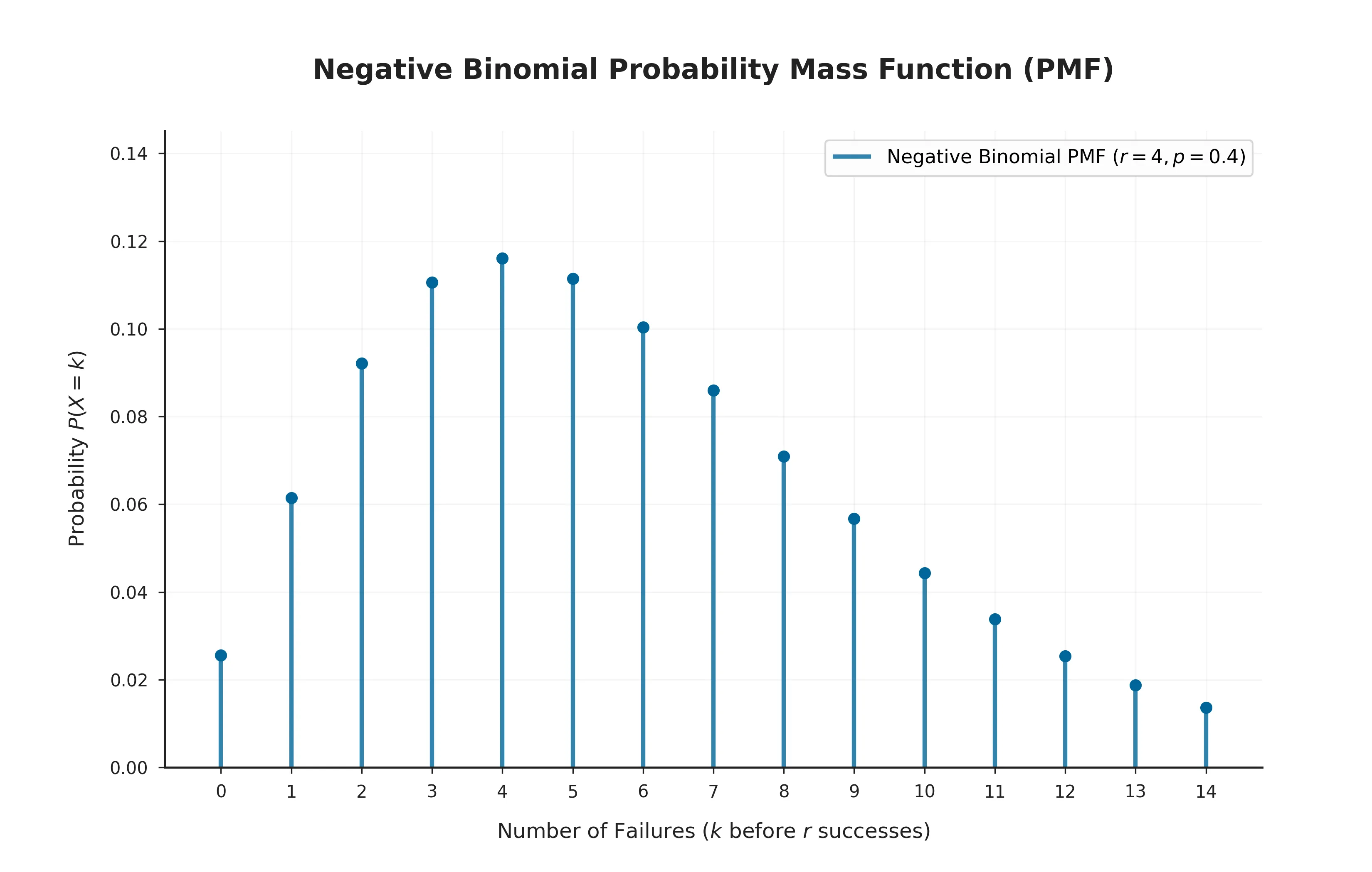
What Is a Negative Binomial Distribution?
In probability theory and statistics, the negative binomial distribution is the discrete probability distribution of the number of failures that occur before a fixed number \( r \) of successes is reached, in a sequence of independent trials where each trial has only two possible outcomes - success or failure - and the same success probability \( p \) on every trial. It answers a question that is, in a sense, the mirror image of the binomial distribution's question: instead of fixing the number of trials and counting successes, the negative binomial distribution fixes the number of successes desired and counts how many failures accumulate along the way. See the formula below for the precise mathematical definition.
The negative binomial distribution generalizes the geometric distribution, which answers the same kind of question for a single success (\( r=1 \)): waiting for the first head is geometric, waiting for the fifth head is negative binomial. Beyond its original trial-counting interpretation, the negative binomial distribution is also one of the most common models for overdispersed count data - counts whose variance exceeds their mean - making it a standard alternative to the Poisson distribution in fields from insurance to genomics (see Where It Shows Up).
The Formula
The probability mass function (PMF) of a negative binomial distribution, which gives the probability of observing exactly \( k \) failures before the \( r \)-th success, is:
\[ P(X = k) = \binom{k+r-1}{k} p^r (1-p)^{k}, \qquad k = 0, 1, 2, \ldots \]where \( \binom{k+r-1}{k} = \dfrac{(k+r-1)!}{k!(r-1)!} \) is a binomial coefficient that counts the number of distinct ways to arrange \( k \) failures among the first \( k+r-1 \) trials, given that the very last trial - the \( (k+r) \)-th - must be the \( r \)-th success. The formula has a direct interpretation: \( p^r \) is the probability of the \( r \) successes, \( (1-p)^{k} \) is the probability of the \( k \) failures, and the binomial coefficient accounts for every possible ordering of those failures and successes among the first \( k+r-1 \) trials, since the final trial's outcome is fixed by definition.
Setting \( r=1 \) collapses the formula to \( P(X=k) = p(1-p)^{k} \), exactly the geometric PMF: the negative binomial distribution is the geometric distribution's natural generalization from one success to \( r \). Unlike the binomial distribution, whose support is the finite set \( \{0,1,\ldots,n\} \), the negative binomial distribution's support is unbounded above - in principle, an arbitrarily long run of failures could precede the \( r \)-th success - though the probabilities still sum to exactly \( 1 \) over all \( k = 0, 1, 2, \ldots \)
Notation & Parameters
A negative binomial distribution with target number of successes \( r \) and success probability \( p \) is written compactly as:
\[ X \sim \operatorname{NegBinomial}(r, p) \quad \text{or equivalently} \quad X \sim \operatorname{NB}(r, p) \]read as "\( X \) follows a negative binomial distribution with target \( r \) successes and success probability \( p \)." Two parameters fully specify the distribution:
- \( r \) is the number of successes to reach, conventionally a fixed positive integer, \( r \ge 1 \), though the PMF extends to any real \( r > 0 \) using the gamma function in place of the factorial (see Estimating Parameters from Data).
- \( p \) is the success probability on each individual trial, satisfying \( 0 < p \le 1 \), and identical across all trials.
- The support of the distribution - the set of values \( X \) can take - is the infinite set of non-negative integers \( \{0, 1, 2, \ldots\} \), making the negative binomial distribution discrete but, unlike the binomial distribution, unbounded above.
- A common alternative parameterization counts the total number of trials \( Y = X + r \) rather than just the failures \( X \); the two forms describe the same experiment and shift by the constant \( r \), so care is needed when comparing formulas across sources or software libraries.
- As with the binomial distribution, the trials are assumed i.i.d. (independent and identically distributed): independence across trials and an identical success probability \( p \) on every trial. If either assumption fails, the resulting count is no longer exactly negative binomial.
Core Properties
The negative binomial distribution inherits its descriptive properties - mean, variance, skewness, kurtosis - directly from the fact that it is a sum of \( r \) independent geometric variables, each contributing its own share of failures to the total.
Mean (Expected Value)
The expected value of a negative binomial random variable follows directly from linearity of expectation applied to a sum of \( r \) geometric\( (p) \) variables:
\[ E[X] = \frac{r(1-p)}{p} \]Intuitively, if each success requires an expected \( (1-p)/p \) failures to arrive (the geometric mean expressed in failure-counting form), then reaching \( r \) successes requires \( r \) times that many failures on average. This identity underlies the moment-based estimation of \( p \) described in Estimating Parameters from Data.
Variance
Because the underlying trials are independent, variances add directly, and the variance of a negative binomial random variable is \( r \) times the variance of a single geometric count:
\[ \operatorname{Var}(X) = \frac{r(1-p)}{p^2} \]Dividing variance by mean gives \( \operatorname{Var}(X)/E[X] = 1/p \), a ratio strictly greater than \( 1 \) whenever \( p < 1 \). This is the formal reason the negative binomial distribution is described as overdispersed: its variance always exceeds its mean, in contrast to the Poisson distribution, whose variance always equals its mean exactly (see Related Distributions). The standard deviation is the square root of the variance, \( \operatorname{SD}(X) = \sqrt{r(1-p)}/p \).
Skewness
Skewness measures the asymmetry of a distribution. For a negative binomial distribution it is:
\[ \text{Skewness} = \frac{2-p}{\sqrt{r(1-p)}} \]For any fixed \( p \) strictly between \( 0 \) and \( 1 \), skewness shrinks toward \( 0 \) as \( r \) grows, since the denominator scales with \( \sqrt{r} \) while the numerator stays fixed. As with the binomial distribution, this is an early hint of the normal approximation for large \( r \), even though the negative binomial distribution's right-skewed, unbounded support keeps it visibly asymmetric for small or moderate \( r \).
Kurtosis
Kurtosis describes the shape of a distribution's tails relative to its center. For a negative binomial distribution, the excess kurtosis is:
\[ \text{Excess kurtosis} = \frac{6}{r} + \frac{p^2}{r(1-p)} \]Both terms shrink toward \( 0 \) as \( r \) grows large for fixed \( p \), so excess kurtosis approaches the value of \( 0 \) that characterizes the normal distribution, mirroring the same large-\( r \) convergence seen in skewness above.
Mode
The mode - the most probable number of failures - is given by \( \left\lfloor \dfrac{(r-1)(1-p)}{p} \right\rfloor \) for \( r > 1 \), and is \( 0 \) whenever \( r = 1 \) (matching the geometric distribution's mode of zero failures). Unlike the symmetric bimodal case that can occur for the binomial distribution, the negative binomial mode is a single value except at specific boundary combinations of \( r \) and \( p \).
Shape as r and p Vary
The two parameters \( r \) and \( p \) control the shape of the negative binomial PMF in distinct, complementary ways, and seeing how the distribution deforms as each one changes builds useful intuition before moving to formal approximations.
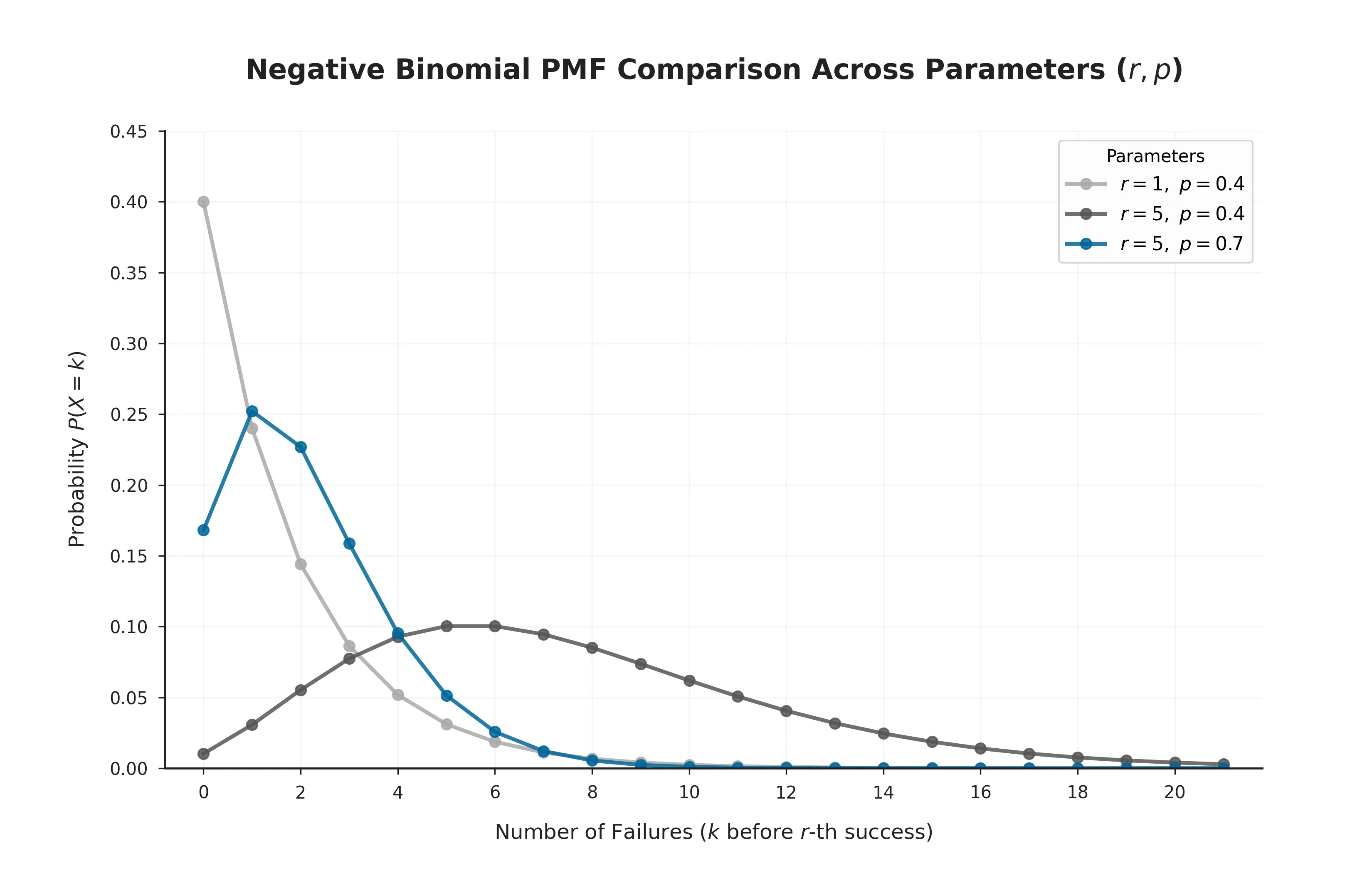
- Increasing \( r \) with \( p \) fixed shifts the distribution's mass to the right, spreads it over a wider range of possible failure counts, and, per the skewness and kurtosis formulas above, makes the shape progressively more symmetric and bell-like, consistent with the normal approximation.
- Increasing \( p \) with \( r \) fixed shrinks the expected number of failures needed to reach \( r \) successes, pulling the distribution's mass toward \( 0 \) and shortening its right tail, since each trial is now more likely to succeed.
- Decreasing \( p \) toward \( 0 \) with \( r \) fixed stretches the distribution's tail dramatically, since failures become far more likely than successes and the wait for the \( r \)-th success grows correspondingly long.
- For \( r=1 \), the distribution reduces to the strictly decreasing, always right-skewed geometric distribution; the characteristic hump seen for larger \( r \) only emerges once \( r \ge 2 \).
Moments & Generating Functions
The moment generating function (MGF) of a negative binomial random variable follows directly from the MGF of a single geometric count, raised to the \( r \)-th power, since the MGF of a sum of independent variables is the product of their individual MGFs:
\[ M(t) = E\left[e^{tX}\right] = \left[\frac{p}{1-(1-p)e^{t}}\right]^r, \qquad t < -\ln(1-p) \]Differentiating \( M(t) \) and evaluating at \( t=0 \) recovers the mean \( r(1-p)/p \) and, together with the second derivative, the variance \( r(1-p)/p^2 \), matching the direct calculations in Core Properties.
The related probability generating function, more commonly used for discrete distributions, is similarly the \( r \)-th power of the geometric probability generating function:
\[ G(z) = E[z^X] = \left[\frac{p}{1-(1-p)z}\right]^r, \qquad |z| < \frac{1}{1-p} \]This "raise the single-success function to the \( r \)-th power" pattern directly parallels the binomial distribution's moment generating function, and is a direct consequence of summing \( r \) independent, identically distributed geometric variables.
Cumulative Distribution Function
The cumulative distribution function (CDF), \( F(k) = P(X \le k) \), gives the probability that a negative binomial variable takes a value at or below a given threshold. It is obtained by summing the PMF over all failure counts from \( 0 \) up to \( k \):
\[ F(k) = P(X \le k) = \sum_{i=0}^{\lfloor k \rfloor} \binom{i+r-1}{i} p^r (1-p)^{i} \]Because the support is unbounded above, the negative binomial CDF is an infinite staircase with a jump at every non-negative integer \( k \), each of height \( P(X=k) \), that approaches - but never exactly reaches - \( 1 \) only in the limit as \( k \to \infty \), unlike the binomial CDF's finite staircase of \( n+1 \) steps. In closed form, \( F(k) \) can also be written using the regularized incomplete beta function, \( F(k) = I_{p}(r, k+1) \), a relationship exploited by statistical software to evaluate negative binomial probabilities without summing every term individually.
Worked Example
Suppose the same online advertisement from the Bernoulli worked example is shown to a stream of independent visitors, each clicking with probability \( p = 0.04 \) (a 4% click-through rate), and the advertiser wants to know how many non-clicking visitors to expect before the \( r = 3 \)rd click occurs. Let \( X \sim \operatorname{NegBinomial}(3, 0.04) \) denote the number of non-clicking visitors shown before the third click. What are the mean and standard deviation of \( X \), and what is the probability that exactly ten visitors fail to click before the third click arrives?
Step 1 - Mean: using \( E[X] = r(1-p)/p \) from Core Properties:
\[ E[X] = \frac{3 \times 0.96}{0.04} = 72 \]Step 2 - Variance and standard deviation: using \( \operatorname{Var}(X) = r(1-p)/p^2 \):
\[ \operatorname{Var}(X) = \frac{3 \times 0.96}{0.04^2} = 1800, \qquad \operatorname{SD}(X) = \sqrt{1800} \approx 42.4 \]Step 3 - Probability of exactly ten non-clicks before the third click: using the PMF with \( k=10 \):
\[ P(X=10) = \binom{12}{10}(0.04)^3(0.96)^{10} = 66 \times 0.000064 \times 0.6648 \approx 0.00281 \]There is roughly a 0.28% chance that exactly ten visitors fail to click before the third one clicks - a low probability, since the expected wait of 72 non-clicks is far larger than 10. This large gap between the mean and the queried value \( k=10 \) illustrates why, with a small success probability like \( p=0.04 \), the bulk of the distribution's mass sits far out along its long right tail rather than near \( 0 \).
Estimating Parameters from Data
When the number of target successes \( r \) is known in advance - as in the sequential-trial setting above - the success probability \( p \) can be estimated from an observed count of failures \( X = k \) using the method-of-moments estimator that inverts the mean formula \( E[X] = r(1-p)/p \):
\[ \hat{p} = \frac{r}{r+k} \]This estimator is consistent, in the sense that it converges to the true \( p \) as more trials are observed, though it is only approximately - not exactly - unbiased for finite samples, unlike the analogous binomial estimator \( \hat p = k/n \).
A more delicate estimation problem arises when the negative binomial distribution is used to model overdispersed count data (see Where It Shows Up) and both \( r \) and \( p \) must be estimated from a sample of counts, with \( r \) no longer restricted to integers. In this setting, \( r \) is typically estimated by maximum likelihood using the gamma-function form of the PMF, since simple closed-form estimators are not generally available; statistical software such as R's MASS::glm.nb() or Python's statsmodels.discrete.discrete_model.NegativeBinomial handle this numerical optimization internally.
Poisson & Normal Approximations
Two well-known approximations to the negative binomial distribution are used depending on how its parameters behave, one that reveals its deep connection to the Poisson distribution and one that applies for large \( r \).
Poisson Limit (Gamma-Poisson Mixture)
The negative binomial distribution can be constructed exactly as a gamma-Poisson mixture: if the Poisson rate \( \lambda \) is itself treated as random, drawn from a \( \operatorname{Gamma}(r, \beta) \) distribution, and \( X \mid \lambda \sim \operatorname{Poisson}(\lambda) \), then the marginal distribution of \( X \) is exactly negative binomial with \( p = \beta/(1+\beta) \). This representation is the formal reason the negative binomial distribution fits overdispersed counts so well: it is, in effect, "Poisson data with a Poisson rate that itself varies across observations."
Normal Approximation
When \( r \) is reasonably large, the central limit theorem - applied to the sum of \( r \) independent geometric variables - implies that a negative binomial random variable is approximately normally distributed with matching mean and variance:
\[ X \approx \mathcal{N}\!\left(\frac{r(1-p)}{p},\ \frac{r(1-p)}{p^2}\right) \]As with the binomial normal approximation, accuracy improves with a continuity correction of \( \pm 0.5 \), and the approximation is most reliable when \( r \) is large and \( p \) is not too close to \( 0 \), which would otherwise leave the distribution heavily right-skewed.
Sums of Negative Binomial Variables
The negative binomial distribution has a closure property directly analogous to the binomial distribution's closure under addition: if \( X_1 \sim \operatorname{NegBinomial}(r_1, p) \) and \( X_2 \sim \operatorname{NegBinomial}(r_2, p) \) are independent and share the same success probability \( p \), their sum is again negative binomial:
\[ X_1 + X_2 \sim \operatorname{NegBinomial}(r_1 + r_2,\ p) \]This follows immediately from viewing each negative binomial variable as a sum of independent geometric\( (p) \) counts: adding \( X_1 \) and \( X_2 \) is the same as pooling \( r_1 + r_2 \) target successes under one combined waiting process. As with the binomial case, the shared \( p \) is essential; if the two variables have different success probabilities, their sum is generally not negative binomial.
Generating Negative Binomial Random Numbers
Because a negative binomial variable is, by construction, a sum of \( r \) independent geometric counts, one direct way to generate one is to simulate \( r \) independent geometric draws and add them together:
- For each of \( j = 1, \ldots, r \), simulate an independent geometric\( (p) \) count \( G_j \) - the number of failures before the first success in a Bernoulli\( (p) \) sequence.
- Return \( X = \sum_{j=1}^{r} G_j \) as the negative binomial draw.
This direct approach becomes computationally wasteful for large \( r \), and does not extend naturally to the non-integer \( r \) used in overdispersion modeling. Statistical software instead typically exploits the gamma-Poisson mixture representation: draw a rate \( \lambda \sim \operatorname{Gamma}(r, \beta) \), then draw \( X \mid \lambda \sim \operatorname{Poisson}(\lambda) \), which works for any real \( r > 0 \) and avoids simulating individual trials entirely.
In practice, these details are handled internally: for example, NumPy's numpy.random.negative_binomial(r, p) and SciPy's scipy.stats.nbinom.rvs(r, p) both return draws from a NegBinomial\( (r, p) \) distribution without requiring the underlying mixture or trial simulation to be implemented by hand.
A Short History
The negative binomial distribution's name reflects an algebraic origin as much as a probabilistic one: its PMF terms arise from expanding \( p^r(1-(1-p))^{-r} \) via the binomial series for a negative exponent, in contrast to the ordinary positive-integer binomial expansion behind the binomial distribution. Early work on waiting times for repeated successes in sequences of trials traces to the same eighteenth-century probabilists who studied the geometric distribution, with the distribution's formal treatment as a distinct object developing over the eighteenth and nineteenth centuries alongside the broader theory of games of chance.
The distribution's modern prominence owes much to its role as an overdispersed alternative to the Poisson distribution. In the early twentieth century, statisticians studying accident and epidemic data - notably in biometrics and public health - found that Poisson models routinely underestimated the variance of observed counts, and the gamma-Poisson mixture construction (see Poisson & Normal Approximations) was developed as a principled way to accommodate this extra variability, cementing the negative binomial distribution's place as a standard tool for count data with unequal underlying rates.
Where It Shows Up
Any scenario reducible to "how many failures occur before a fixed number of successes" is, in principle, negative binomial in its original trial-counting sense - but its far more common modern use is as a flexible model for overdispersed counts. A selection of concrete examples across statistics, insurance, and machine learning:
- Insurance claims modeling - the number of claims filed by a policyholder in a given period is classically modeled as negative binomial rather than Poisson, since claim counts typically show variance well in excess of their mean across a heterogeneous population of policyholders.
- Epidemiology and public health - counts of disease cases across regions or time periods, and the number of secondary infections generated by an index case in outbreak modeling, are commonly fit with negative binomial regression to capture overdispersion driven by unobserved heterogeneity in exposure or susceptibility.
- RNA-sequencing and genomics - read counts per gene across biological replicates are a textbook case of overdispersed count data, and negative binomial models underlie widely used differential expression tools such as DESeq2 and edgeR.
- Sequential quality testing - in its original waiting-time sense, the number of defective items inspected before finding a fixed number of acceptable ones (or vice versa) follows a negative binomial distribution.
- Sports and games analytics - the number of games played, or misses recorded, before a team or player achieves a fixed number of wins or successes is a standard negative binomial modeling exercise, directly extending the geometric distribution's single-success case.
- Natural language processing - word and n-gram frequency counts across documents are frequently overdispersed relative to a Poisson assumption, motivating negative binomial (or related mixture) models in text analytics and topic modeling.
- Web and app analytics - the number of page visits, purchases, or app sessions per user over a fixed period often shows more variance across users than a Poisson model allows for, making the negative binomial distribution a common choice for user-level count modeling.
- Ecology - counts of organisms per sampling quadrat, such as insects per trap or plants per plot, are a long-standing application of the negative binomial distribution in population ecology, reflecting spatial clustering that a Poisson model cannot capture.
As with the binomial distribution, the negative binomial model is occasionally misapplied when its core assumptions - independence across trials or observations, and a constant success probability \( p \) - are violated in ways the added dispersion parameter cannot fully absorb; in such cases, zero-inflated or hurdle extensions of the negative binomial are often used instead (see Related Distributions).
Frequently Asked Questions
- It is the probability distribution of the number of failures (or, in an equivalent form, the total number of trials) that occur before a fixed number of successes, r, is reached in a sequence of independent trials, each with the same success probability p.
- A binomial distribution fixes the number of trials n and treats the number of successes as random. A negative binomial distribution fixes the number of successes r and treats the number of trials (or failures) needed to reach that target as random; the two distributions ask complementary questions about the same sequence of Bernoulli trials.
- For a negative binomial random variable X counting failures before r successes with success probability p, the mean is E[X] = r(1 - p)/p and the variance is Var(X) = r(1 - p)/p^2. Because the variance always exceeds the mean by a factor of 1/p, the negative binomial distribution is naturally overdispersed relative to the Poisson.
- The geometric distribution is the special case of the negative binomial distribution with r = 1: a negative binomial random variable with parameters r and p can be constructed as the sum of r independent geometric(p) random variables.
- The Poisson distribution constrains its variance to equal its mean, which real count data frequently violates through overdispersion. The negative binomial distribution relaxes this constraint by adding a dispersion parameter, making it a common default for modeling overdispersed counts such as insurance claims or word frequencies.
- Yes. While the original trial-counting interpretation requires r to be a positive integer, the negative binomial probability mass function is well defined for any real r > 0 using the gamma function in place of the factorial, an extension routinely used in negative binomial regression.
- It is discrete: the random variable counts whole-number failures or trials and can take any non-negative integer value with no upper bound, so probability is described by a probability mass function rather than a probability density function.
- The geometric distribution is the special case of the negative binomial distribution with r = 1, the binomial distribution answers the complementary question of successes in a fixed number of trials, the negative binomial arises as a gamma-Poisson mixture that generalizes the Poisson distribution, and the normal distribution approximates it for large r via the central limit theorem.